Axes and Antipodal Symmetry

Directions vs. Axes

In MTEX it is possible to consider three dimensional vectors either as directions or as axes. The key option to distinguish between both interpretations is antipodal.

Consider a pair of vectors

v1 = vector3d(1,1,2);
v2 = vector3d(1,1,-2);

and plots them in a spherical projection

plot([v1,v2],'label',{'v_1','v_2'})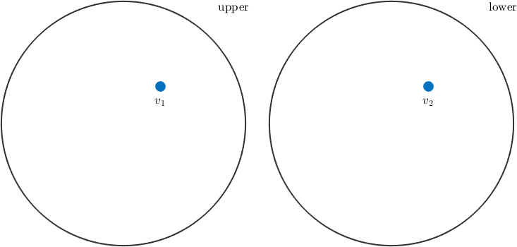

These vectors will appear either on the upper or on the lower hemisphere. In order to treat these vectors as axes, i.e. in order to assume antipodal symmetry - one has to use the keyword antipodal.

plot([v1,v2],'label',{'v_1','v_2'},'antipodal')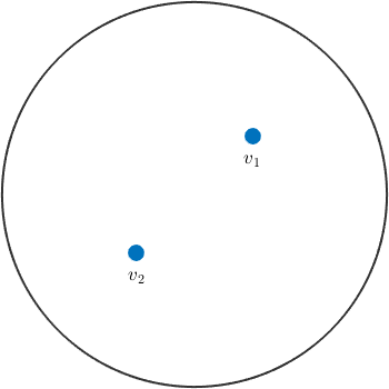

Now the direction v_2 is identified with the direction -v_2 which plots at the upper hemisphere.

The Angle between Directions and Axes

As a consequence the angle between two axes v1, v2 will always be the smallest angle between the directions v1, v2 and v1, -v2, i.e. it will always be smaller than 90 degree. In the absence of antipodal symmetry we obtain

angle(v1,v2) / degree

ans =
  109.4712

whereas, if antipodal symmetry is assumed we obtain

angle(v1,v2,'antipodal') / degree

ans =
   70.5288

Antipodal Symmetry in Density Estimation

Another example, where antipodal symmetry matters is density estimation. For ordinary directions we obtain an arbitrary spherical function

v = vector3d.rand(100)
density = v.calcDensity;
plot(density)

v = vector3d
 size: 100 x 1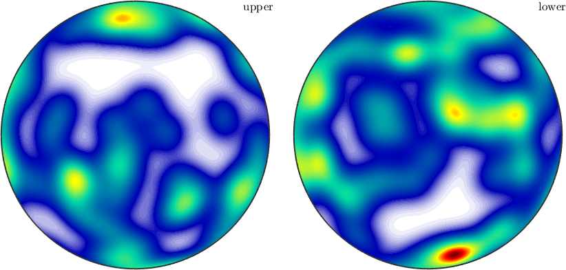

Whereas, if antipodal symmetry is present the resulting density function will have antipodal symmetry as well

density = v.calcDensity('antipodal')
plot(density,'complete')

density = S2FunHarmonic
  bandwidth: 25
  antipodal: true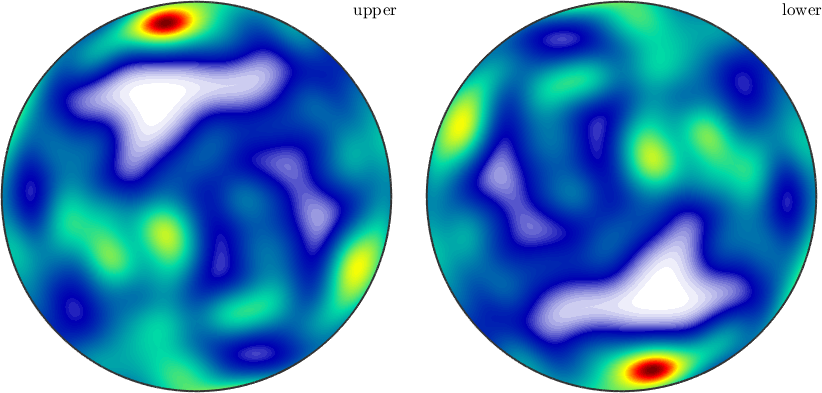
  isReal: true

Antipodal Symmetry in Experimental Pole Figures

Due to Friedel's law experimental pole figures always provide antipodal symmetry. One consequence of this fact is that MTEX plots pole figure data always on the upper hemisphere. Moreover if you annotate a certain direction to pole figure data, it is always interpreted as an axis, i.e. projected to the upper hemisphere if necessary

mtexdata dubna
CS = pf.CS;

% plot the first pole figure
plot(pf({1}))

% annotate a axis on the souther hemisphere
annotate(vector3d(1,0,-1),'labeled','backgroundColor','w')

pf = PoleFigure (xyz)
  crystal symmetry : Quartz (321, X||a*, Y||b, Z||c*)
 
  h = (02-21), r = 72 x 19 points
  h = (10-10), r = 72 x 19 points
  h = (10-11)(01-11), r = 72 x 19 points
  h = (10-12), r = 72 x 19 points
  h = (11-20), r = 72 x 19 points
  h = (11-21), r = 72 x 19 points
  h = (11-22), r = 72 x 19 points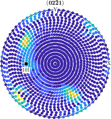

Antipodal Symmetry in Recalculated Pole Figures

However, in the case of pole figures calculated from an ODF antipodal symmetry is in general not present.

% some prefered orientation
o = orientation.byEuler(20*degree,30*degree,0,'ZYZ',CS);

% define an unimodal ODF
odf = unimodalODF(o);

% plot pole figures
plotPDF(odf,[Miller(1,2,2,CS),-Miller(1,2,2,CS)])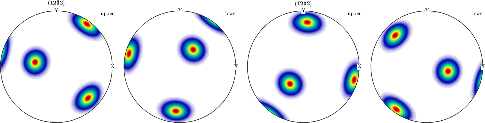

Hence, if one wants to compare calculated pole figures with experimental ones, one has to add antipodal symmetry.

plotPDF(odf,Miller(1,2,2,CS),'antipodal')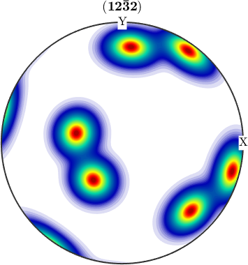

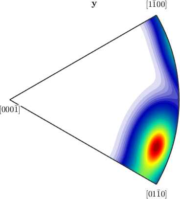
Antipodal Symmetry in Inverse Pole Figures

The same reasoning as above holds true for inverse pole figures. If we look at complete, inverse pole figures they do not posses antipodal symmetry in general

plotIPDF(odf,[yvector,-yvector],'complete')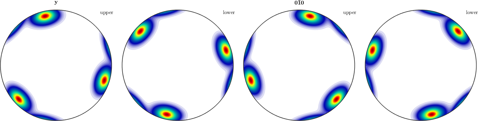

However, if we add the keyword antipodal, antipodal symmetry is enforced.

plotIPDF(odf,yvector,'antipodal','complete')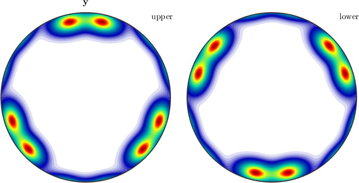

Notice how MTEX, automatically reduces the fundamental region of inverse pole figures in the case that antipodal symmetry is present.

plotIPDF(odf,yvector)

plotIPDF(odf,yvector,'antipodal')