A common way to interpret ODFs is to think of them as superposition of different components that originate from different deformation processes and describe the texture of the material. In this section we describe how these components can be identified from a given ODF.
We start by reconstruction a Quartz ODF from Neutron pole figure data.
% import Neutron pole figure data from a Quartz specimen
mtexdata dubna silent
% reconstruct the ODF
odf = calcODF(pf,'zeroRange');
% visualize the ODF in sigma sections
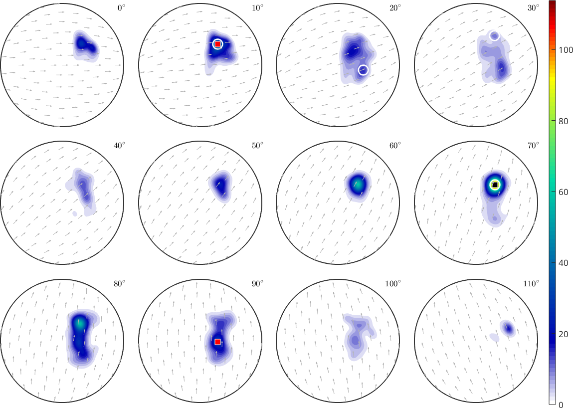
plotSection(odf,'sigma','sections',12,'layout',[3,4])
mtexColorbar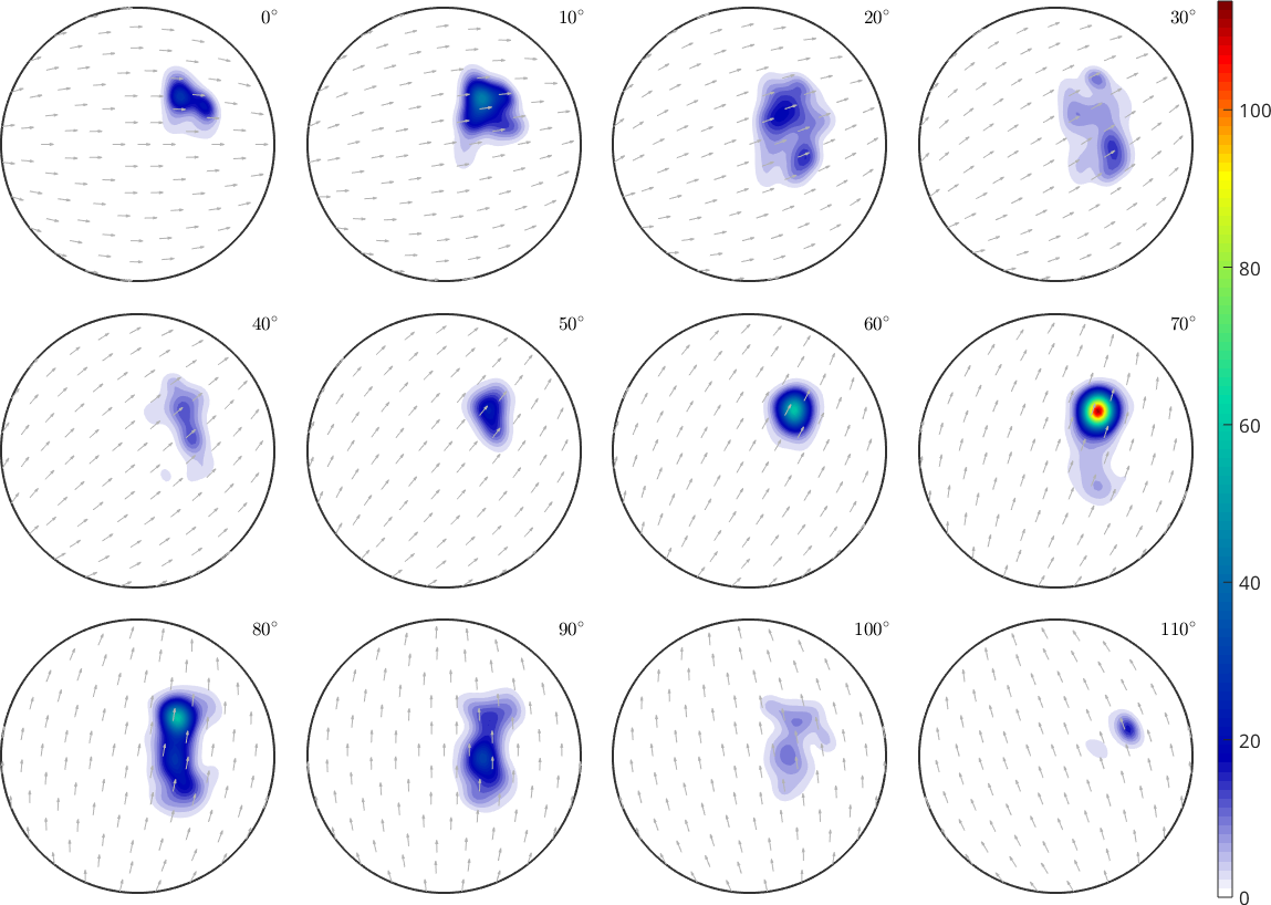
The preferred orientation
First of all we observe that the ODF posses a strong maximum. To find this orientation that corresponds to the maximum ODF intensity we use the max command.
[value,ori] = max(odf)value =
107.4378
ori = orientation (Quartz → y↑→x)
Bunge Euler angles in degree
phi1 Phi phi2
133.216 34.0595 207.735Note that, similarly as the MATLAB max command, the second output argument is the position where the maximum is attained. In our case we observe that the maximum value is about 121. To visualize the corresponding preferred orientation we plot it into the sigma sections of the ODF.
annotate(ori)
We may not only use the command max to find the global maximum of an ODF but also to find a certain amount of local maxima. The number of local maxima MTEX should search for, is specified as by the option 'numLocal', i.e., to find the three largest local maxima do
[value,ori] = max(odf,'numLocal',3)

annotate(ori(2:end),'MarkerFaceColor','red')
value =
107.4378
48.7483
33.3106
ori = orientation (Quartz → y↑→x)
size: 3 x 1
Bunge Euler angles in degree
phi1 Phi phi2
133.216 34.0595 207.735
139.269 37.9594 257.881
83.1396 32.8648 329.847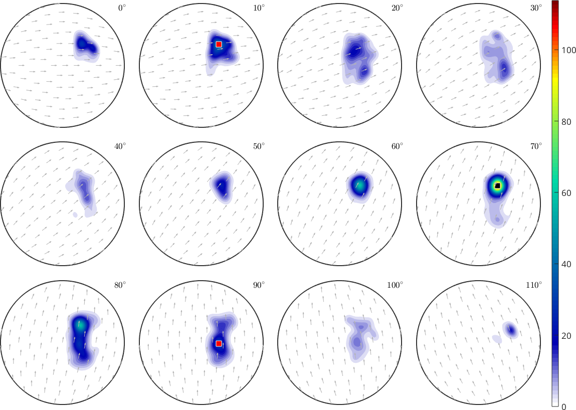
Note, that orientations are returned sorted according to their ODF value.
Volume Portions
It is important to understand, that the value of the ODF at a preferred orientation is in general not sufficient to judge the importance of a component. Very sharp components may result in extremely large ODF values that represent only very little volume. A more robust and physically more relevant quantity is the relative volume of crystal that have an orientation close to the preferred orientation. This volume portion can be computed by the command volume(odf,ori,delta) where ori is a list of preferred orientations and delta is the maximum disorientation angle. Multiplying with \(100\) the output will be in percent
delta = 10*degree;
volume(odf,ori,delta) * 100
ans =
10.0306
5.2569
3.2151We observe that the sum of all volume portions is far from \(100\) percent. This is very typical. The reason is that the portion of the full orientations space that is within the \(10\) degree disorientation distance from the preferred orientations is very small. More precisely, it represents only
volume(uniformODF(odf.CS),ori(1),delta) * 100ans =
0.1690percent of the entire orientations space. Putting these values in relation it becomes clear, that all the components are multiple times stronger than the uniform distribution. We may compute these factors by
volume(odf,ori,delta) ./ volume(uniformODF(odf.CS),ori,delta)ans =
59.3618
31.1107
19.0272It is important to understand, that all these values above depend significantly from the chosen disorientation angle delta. If delta is chosen too large
delta = 40*degree
volume(odf,ori,delta)*100
delta =
0.6981
ans =
54.2401
39.6253
37.9830it may even happen that the components overlap and the sum of the volumes exceeds 100 percent.
Non circular components
A disadvantage of the approach above is that one is restricted to circular components with a fixed disorientation angle which makes it hard to analyze components that are close together. In such settings one may want to use the command calcComponents. This command starts with evenly distributed orientations and lets the crawl towards the closest preferred orientation. At the end of this process the command returns these preferred orientation and the percentage of orientations that crawled to each of them.
[ori, vol] = calcComponents(odf);
ori
vol * 100
ori = orientation (Quartz → y↑→x)
size: 8 x 1
Bunge Euler angles in degree
phi1 Phi phi2
133.186 34.1505 207.61
139.383 37.9096 257.72
70.1751 27.4727 285.099
83.1683 32.9499 329.641
107.239 33.4953 205.758
156.696 34.8618 208.613
75.0198 25.698 280.516
108.85 33.6596 206.307
ans =
36.3641
25.7390
19.4891
7.5145
3.2018
2.3516
2.2017
1.6386These volumes always sums up to approximately 100 percent. While the preferred orientations should be the same as those computed by the max command.
annotate(ori,'MarkerFaceColor','none','MarkerEdgeColor','white',...
  'linewidth',2,'MarkerSize',15,'marker','o')