Axis Distribution Function

A misorientation has an axis and an angle. The axis distribution function (ADF) keeps the crystal direction about which the rotation occurs and integrates out the angle. It is the spherical counterpart of the angle distribution and a marginal of the misorientation distribution function (MDF).

MTEX represents an ADF by an S2Fun. Start with Theory of Misorientations if symmetry-equivalent rotations and the fundamental region are unfamiliar. The kernel smoothing used below is introduced in Density Estimation.

The axis distribution of random orientations

Random crystal orientations do not produce a constant ADF. Crystal symmetry restricts every misorientation to a fundamental region. The largest permitted angle depends on the axis direction, so some axes represent more rotations than others.

calcAxisDistribution computes this symmetry-only reference. Point group 432 gives the cubic example.

cs = crystalSymmetry('432');

adf = calcAxisDistribution(cs)

adf = S2FunHarmonicSym (432)
  bandwidth: 256
  antipodal: true

Like any spherical function, adf can be plotted, evaluated, and integrated. The convenience command plotAxisDistribution draws the same density. Passing both symmetries describes a same-phase pair, while antipodal applies grain exchange symmetry.

plotAxisDistribution(cs,cs,'antipodal')
mtexColorbar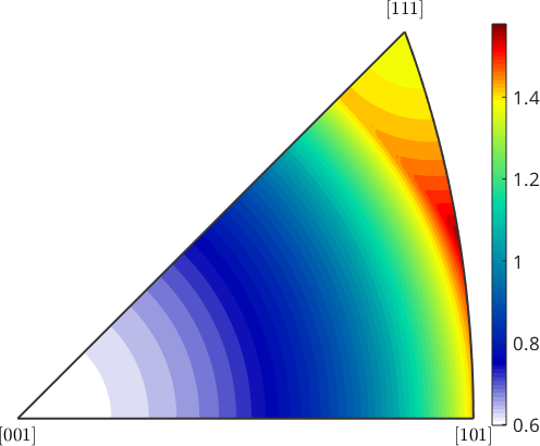

The light \([001]\) corner is the minimum. The red band towards the \([101]\)-- \([111]\) edge is more probable because the fundamental region extends to larger angles there.

MTEX normalizes a density to have mean one. The numerical range and its ratio quantify the variation visible in the colour scale.

uniformRange = [min(adf),max(adf)]
uniformRatio = uniformRange(2) ./ uniformRange(1)

uniformRange =
    0.5974    1.5652
uniformRatio =
    2.6198

The density runs from 0.597 to 1.565 multiples of the mean, a factor of 2.620. A measured ADF must therefore be compared with this reference, not with a constant.

The axis distribution of boundary misorientations

A grain is a phase-homogeneous, spatially connected region of EBSD pixels produced by segmentation. A grain boundary is a segment between two neighbouring pixels that belong to different grains. Load the magnesium map, segment its indexed pixels at \(5^\circ\), and smooth the boundary geometry for five iterations. The plotting convention states the specimen frame used by this data set.

plottingConvention.default('y↑→x');
mtexdata twins silent

grains = calcGrains(ebsd('indexed'),'angle',5*degree);
grains = smoothBoundary(grains,5);

% retain boundaries between magnesium grains
gB = grains.boundary('Magnesium','Magnesium');
mori = gB.misorientation;

axis selects the smallest-angle symmetry-equivalent representative and returns its axis in the crystal frame. The summary reports one axis for each of the 2803 boundary segments.

axesCrystal = axis(mori)

axesCrystal = Miller (Magnesium)
 size: 2803 × 1

Each boundary segment contributes once by default. Passing its segLength as a weight instead estimates a distribution by boundary trace length. The \(5^\circ\) halfwidth controls the spherical kernel smoothing.

plotAxisDistribution(mori,'contourf','halfwidth',5*degree,...
  'weights',gB.segLength)
mtexColorbar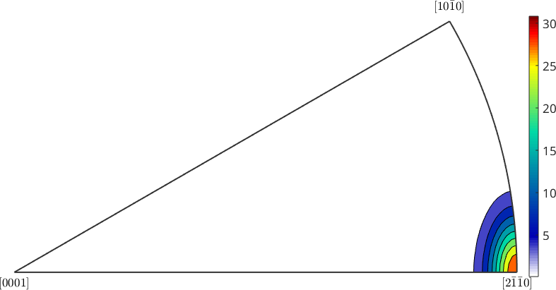

The isolated maximum is the extension-twin prism axis. Computing the underlying spherical density returns a peak of 30.8 multiples of the mean and prints the indexed direction at that peak.

[peakDensity,twinAxis] = max(calcDensity(axesCrystal,...
  'halfwidth',5*degree,'weights',gB.segLength));

peakDensity
indexedTwinAxis = round(twinAxis)

peakDensity =
   30.8183
 
indexedTwinAxis = Miller (Magnesium)
 antipodal: true
  h  k  i  l
  2 -1 -1  0

The symmetry-only reference for magnesium

Use the two symmetries stored with the misorientation to plot the random reference for the same problem.

plotAxisDistribution(mori.CS,mori.SS,'antipodal')
mtexColorbar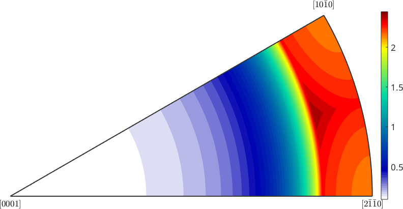

This reference is not essentially flat. It has the broad variation caused by hexagonal symmetry, but it has no isolated peak at the twin axis. The comparison separates a preferred boundary relationship from the geometry of the misorientation fundamental region.

An ADF has discarded the angle, so an axis peak alone does not identify a twin law. Confirm the complete misorientation against the ideal relation, as in Twinning.

Crystal versus specimen coordinates

A reference frame is the coordinate system in which data are expressed; it is distinct from the symmetry attached to it. The crystal frame is fixed to the lattice, whereas the specimen frame is fixed to the sample. The crystal-coordinate ADF above asks which lattice direction is the axis.

Passing two orientations separately to plotAxisDistribution asks where that axis points in the specimen frame. The two EBSD ids stored for every segment recover the orientations on its two sides.

ori1 = ebsd(gB.ebsdId(:,1)).orientations;
ori2 = ebsd(gB.ebsdId(:,2)).orientations;

plotAxisDistribution(ori1,ori2,'contourf','halfwidth',5*degree,...
  'weights',gB.segLength)
mtexColorbar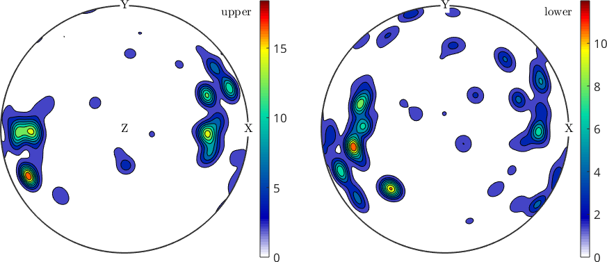

The directed axes occupy the full sphere because the stored first and second sides fix an order and the specimen symmetry is trivial. The single crystal direction becomes several specimen-frame clusters because each grain carries that lattice direction into a different sample direction.

For an unordered same-phase population, add antipodal to identify opposite specimen directions. Tilt and Twist Boundaries uses the specimen-coordinate axis to classify boundaries.

The texture-dependent uncorrelated reference

There are three distinct comparisons. The measured boundary ADF is correlated because its grains touch. A symmetry-only ADF assumes random orientations. Between them lies the uncorrelated ADF predicted by the measured texture when grain orientations are paired independently.

Estimate the magnesium ODF from grain mean orientations. Area weights make this a sampled-area texture rather than a one-grain-one-vote texture. The Fourier flag selects the harmonic representation used efficiently by calcMDF.

mgGrains = grains('Magnesium');
odf = calcDensity(mgGrains.meanOrientation,'weights',mgGrains.area,...
  'halfwidth',10*degree,'Fourier');
mdf = calcMDF(odf);

adfTexture = calcAxisDistribution(mdf);

plot(adfTexture,'upper','antipodal')
mtexColorbar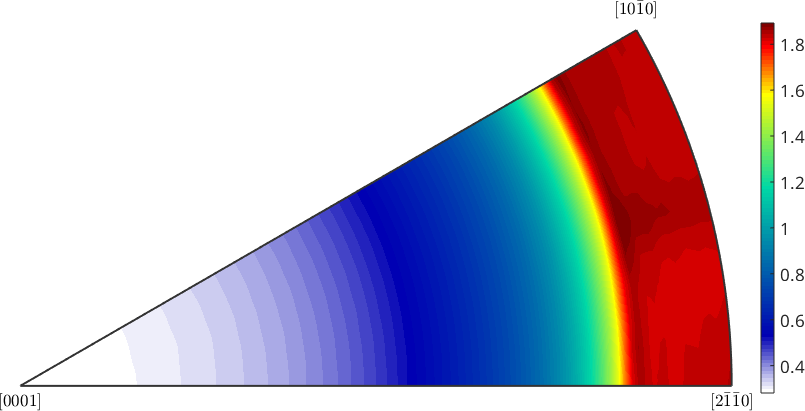

The texture-dependent reference has broad symmetry-related maxima, but it lacks the boundary distribution's sharp twin-axis peak. Texture alone, under independent pairing, therefore does not explain that boundary population.

Axis and angle remain coupled in the MDF

The ADF and angle distribution are separate marginals. Peaks in the two plots need not belong to the same misorientations, and the two marginals cannot reconstruct the full MDF.

For an MDF \(f(\mathbf{h},\omega)\), MTEX evaluates the full-angle ADF as

\[A(\mathbf{h}) = \frac{2N}{\pi}\int_0^{\omega_{\max}(\mathbf{h})} f(\mathbf{h},\omega)\sin^2(\omega/2)\,\mathrm{d}\omega.\]

Here \(\mathbf{h}\) is the axis, \(\omega\) is the angle, and \(N\) accounts for the symmetry copies represented by the fundamental region. The upper limit \(\omega_{\max}(\mathbf{h})\) is why a uniform MDF has a non-constant ADF.

calcAxisDistribution accepts minAngle and maxAngle to study an angle window. Its resolution option is the angular quadrature step; reduce it when a narrow window must be integrated to better than percent accuracy.

The axis-angle description is singular at zero angle. Small orientation errors can therefore produce large axis errors for low-angle rotations. Restrict the angle range before interpreting a low-angle axis maximum.

References

Next

Angle Distribution keeps the angle and integrates out the axis. Return to Misorientation Distribution Function when the coupling between axis and angle matters. Continue to Grain Boundaries when the boundary plane and trace must be considered as well.

References

- A. Morawiec, Distributions of Misorientation Angles and Misorientation Axes for Crystallites with Different Symmetries, Acta Crystallographica A 53 (1997), 273--285.
- F. Basson, Probabilities of Random Disorientation Axes in Cubic Polycrystals, Journal of Applied Crystallography 30 (1997), 102--106.
- A. Morawiec, Orientations and Rotations: Computations in Crystallographic Textures, Springer, 2004, chapter 7.
- A. Morawiec, On the Magnitude of Error in the Determination of Rotation Axes, Journal of Applied Crystallography 57 (2024), 1059--1066.