Angle Distribution Function

A misorientation contains a rotation axis and a rotation angle. The misorientation angle distribution keeps only the disorientation angle \(\omega\). It is the one-dimensional marginal obtained by integrating out the axis of the misorientation distribution function (MDF).

This compact summary answers "how far apart are the crystal orientations?" It does not answer "about which axis?" The latter question is treated in the companion Axis Distribution page.

First read misorientation theory and grain reconstruction. The final comparison also uses kernel density estimation.

Random orientations do not give a flat curve

Even for completely random orientations, disorientation angles are not uniformly distributed. Small angles are rare because few rotations lie close to the identity. Large angles are limited by the shape of the fundamental region.

This reference curve is often called the Mackenzie distribution. Strictly, Mackenzie's result is for cubic symmetry. MTEX computes the analogous random-disorientation baseline for any pair of crystal symmetries with calcAngleDistribution.

cs = crystalSymmetry('432');
[density,omega] = calcAngleDistribution(cs);

close all
plot(omega ./ degree,density,'linewidth',2)
xlabel('misorientation angle (degrees)')
ylabel('relative frequency (mrd)')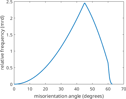

The cubic curve starts at zero because vanishingly small rotations occupy little rotation space. It terminates well below \(180^\circ\) because cubic symmetry supplies a smaller equivalent rotation beyond that limit.

maxAngle returns the largest angle in the fundamental region. For cubic symmetry it is

cubicMaxAngle = maxAngle(cs) ./ degree

cubicMaxAngle =
   62.7994

Symmetry sets the range and the baseline

Fewer symmetry operations leave a larger fundamental region and therefore permit larger distinct disorientation angles.

close all
plotAngleDistribution(crystalSymmetry('1'),'linewidth',2,'figSize','small')
hold on
plotAngleDistribution(crystalSymmetry('622'),'linewidth',2)
plotAngleDistribution(crystalSymmetry('432'),'linewidth',2)
hold off
legend('1','622','432','Location','northwest')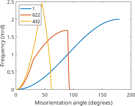

The triclinic curve extends furthest, while the hexagonal and cubic curves end progressively earlier. Their shapes differ as well. A measured curve must therefore be compared with the baseline for its own symmetries.

A misorientation between two different phases has one crystal symmetry on each side. Pass both symmetry objects so that MTEX constructs their joint fundamental region.

close all
plotAngleDistribution(crystalSymmetry('222'),...
  crystalSymmetry('12/m1'),'linewidth',2,'figSize','small')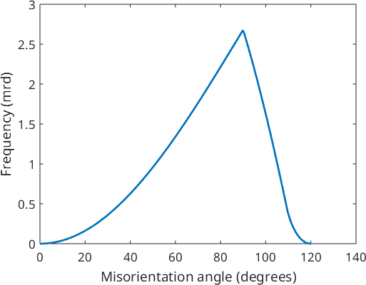

This curve is the random reference for an orthorhombic-to-monoclinic relationship. Its range and shape are set jointly by the two phases, not by either phase alone.

The angle distribution of measured boundaries

Now compare the symmetry-only reference with a measured boundary population. The plotting convention matches the specimen frame stored with the magnesium data set.

plottingConvention.default('y↑→x');
mtexdata twins silent

grains = calcGrains(ebsd('indexed'),'threshold',5*degree);

% misorientations of all magnesium--magnesium boundary segments
mori = grains.boundary('Magnesium','Magnesium').misorientation

mori = misorientation (Magnesium → Magnesium)
  size: 3286 × 1
  antipodal: true

The summary reports 3,286 boundary segments. This is one sample per segment, not one vote per neighbouring grain pair, so a longer boundary contributes more samples. The displayed antipodal: true records grain exchange symmetry. See Grain Exchange Symmetry for why reversing the grains gives an equivalent inverse.

plotAngleDistribution displays the measured angles as a histogram. Adding the random baseline makes the deviation from symmetry alone visible.

close all
plotAngleDistribution(mori,'figSize','small')
hold on
plotAngleDistribution(mori.CS,mori.SS,'linewidth',2)
hold off
legend('boundary misorientations','random orientations')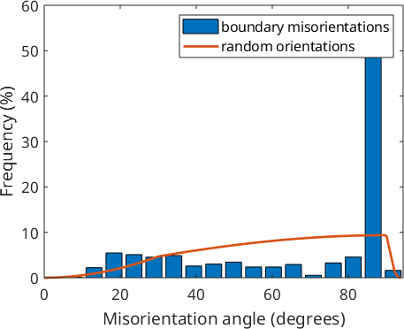

The sharp peak at about \(86^\circ\) is the twin boundary that gives this data set its name. It carries the vast majority of all boundary segments and completely dominates the distribution. The random curve has no corresponding peak.

In this overlay, the histogram bars sum to 100 percent and the reference curve uses the same percent-per-bin scale. A standalone smooth curve uses multiples of a random distribution (mrd) instead.

The numbers behind the histogram are returned by calcAngleDistribution.

[density,omega] = calcAngleDistribution(mori);
[~,peakBin] = max(density);
peakBinAngle = omega(peakBin) ./ degree

peakBinAngle =
   87.1380

The most populated bin is centred at \(87.14^\circ\). This is a histogram bin centre, not a fitted twin angle. The complete twin relationship, including its axis, is tested in Twinning.

Correlated, uncorrelated, and random

The boundary histogram is correlated: it uses only grains that are neighbours. An uncorrelated distribution pairs arbitrary grains from the same data set. It contains the effect of texture but not the effect of which grains became neighbours.

Estimate an ODF from the magnesium grain mean orientations. Each grain contributes once here, regardless of its area. The halfwidth controls the angular smoothing. The explicit harmonic conversion selects an efficient representation for the convolution.

odf = calcDensity(grains('Magnesium').meanOrientation,...
  'halfwidth',10*degree);
mdf = calcMDF(SO3FunHarmonic(odf));

calcMDF pairs the texture with itself to obtain the uncorrelated MDF. Plot its angle marginal between the boundary histogram and the symmetry-only reference.

close all
plotAngleDistribution(mori,'figSize','small')
hold on
plotAngleDistribution(mdf,'linewidth',2)
plotAngleDistribution(mori.CS,mori.SS,'linewidth',2)
hold off
legend('boundary','uncorrelated texture','random orientations')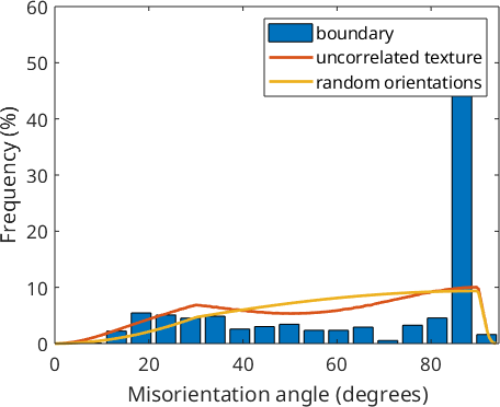

The uncorrelated curve stays close to the uniform-orientation curve. The missing twin peak shows that it belongs to the boundary network, not the texture. The correlated histogram is sharply peaked, whereas both references remain broad.

An angle peak identifies a preferred angular separation, not a complete orientation relationship. Different axes can produce the same angle. Return to the MDF page for the full distribution. Its other marginal is the axis distribution.

References

Next

The next documentation chapter introduces orientation distribution functions, which supply the texture model used for the uncorrelated curve above. For spatially resolved applications, continue with Grain Boundaries.

References

- J. K. Mackenzie, Second Paper on Statistics Associated with the Random Disorientation of Cubes, Biometrika 45 (1958), 229--240. Derives the cubic random baseline.
- H. Grimmer, The Distribution of Disorientation Angles if All Relative Orientations of Neighbouring Grains Are Equally Probable, Scripta Metallurgica 13 (1979), 161--164. Extends the calculation to non-cubic crystal systems.
- A. Morawiec, Orientations and Rotations: Computations in Crystallographic Textures, Springer, 2004. Develops rotation-space geometry and its distributions.
- V. Randle, Grain Boundary Misorientation Distributions, Current Opinion in Solid State and Materials Science 5 (2001), 3--8. Compares angle-only and full misorientation representations for boundary populations.