The following script is a quick guide through the grain reconstruction capabilities of MTEX. It uses the same data set as in the corresponding publication Grain detection from 2d and 3d EBSD data. Data courtesy of Daniel Rutte and Bret Hacker, Stanford.
mtexdata mylonite

% plot a phase map
plot(ebsd)
ebsd = EBSD (y↑→x)
Phase Orientations Mineral Color Symmetry Crystal reference frame
1 3444 (28%) Andesina LightSkyBlue -1 X||a*, Z||c
2 3893 (31%) Quartz DarkSeaGreen -3m1 X||a*, Y||b, Z||c*
3 368 (2.9%) Biotite Goldenrod 2/m11 X||a*, Y||b*, Z||c
4 4781 (38%) Orthoclase LightCoral 12/m1 X||a*, Y||b*, Z||c
Scan unit : um
X x Y x Z : [15000, 24000] x [1020, 3990] x [0, 0]
Normal vector: (0,0,1)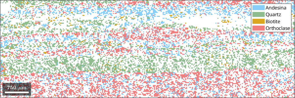
The phase map displays a multi-phase rock specimen with phases such as Andesine, Quartz, Biotite, and Orthoclase. We will now focus on a smaller rectangular region of interest defined by the coordinates [xmin, ymin, xmax - xmin, ymax - ymin].
region = [19000 1500 4000 1500];
% overlay the selected region on the phase map
rectangle('position',region,'edgecolor','k','linewidth',2)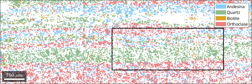
Now copy the EBSD data within the selected rectangle to a new variable
ebsd_region = ebsd(inpolygon(ebsd,region))ebsd_region = EBSD (y↑→x)
Phase Orientations Mineral Color Symmetry Crystal reference frame
1 578 (20%) Andesina LightSkyBlue -1 X||a*, Z||c
2 1144 (40%) Quartz DarkSeaGreen -3m1 X||a*, Y||b, Z||c*
3 58 (2%) Biotite Goldenrod 2/m11 X||a*, Y||b*, Z||c
4 1066 (37%) Orthoclase LightCoral 12/m1 X||a*, Y||b*, Z||c
Scan unit : um
X x Y x Z : [19020, 22980] x [1500, 3000] x [0, 0]
Normal vector: (0,0,1)Grain Reconstruction
Next we reconstruct the grains and grain boundaries in the region of interest, using a 15 degree orientation change threshold.
grains = calcGrains(ebsd_region,'angle',15*degree)

% plot a phase map of the region of interest
plot(ebsd_region)

% overlay the grain boundaries
hold on
plot(grains.boundary,'color','k','linewidth',1.5)
hold off
grains = grain2d (y↑→x)
Phase Grains Pixels Mineral Symmetry Color
1 371 578 Andesina -1 LightSkyBlue
2 189 1144 Quartz -3m1 DarkSeaGreen
3 55 58 Biotite 2/m11 Goldenrod
4 380 1066 Orthoclase 12/m1 LightCoral
boundary segments: 4626 (157002 µm)
inner boundary segments: 1 (45 µm)
triple points: 1333
Properties: meanRotation, GOS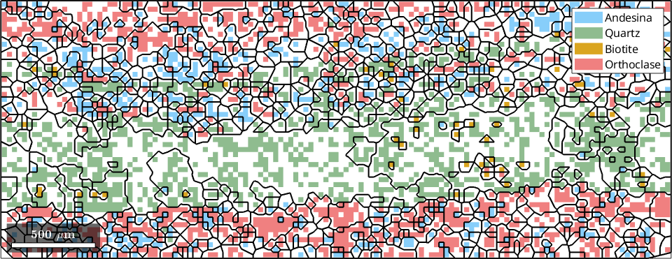
We may also visualize the different quartz orientations together with the grain boundaries.
% plot a phase map of three of the phases based on the grains data
plot(grains({'Andesina','Biotite','Orthoclase'}),'FaceAlpha',0.4)

hold on
% add the quartz orientations as ipf map based on EBSD data
plot(ebsd_region('Quartz'),ebsd_region('Quartz').orientations)

% plot grain boundaries so that those in the Quartz are shown
plot(grains.boundary,'color','black');
legend off
hold off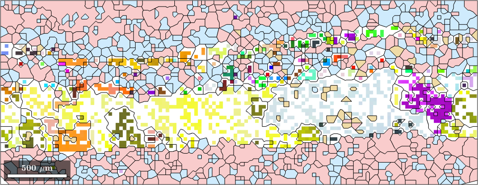
In this visualization most phases are displayed in uniform colors, while Quartz is colored according to the ipf color key
close all
ipfKey = ipfColorKey(ebsd_region('Quartz'));
plot(ipfKey)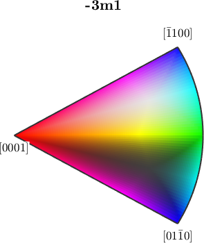
Alternatively, we can display each quartz grain according to its mean orientation.
plot(grains({'Andesina','Biotite','Orthoclase'}),'FaceAlpha',0.4)
hold on
plot(grains('Quartz'),grains('Quartz').meanOrientation)
legend off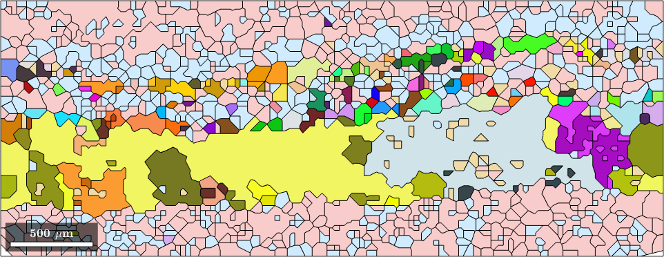
Highlight specific boundaries
We can create a phase map with certain grain boundaries highlighted. In this phase map, we highlight grain boundaries where neighboring grains of Andesine and Orthoclase exhibit a misorientation with a rotational axis close to the c-axis.
close all
% copy all boundaries between Andesina, Orthoclase to a new variable
AOboundary = grains.boundary('Andesina','Orthoclase');
% copy the misorientation angle of this boundary in radians to a new variable.
angle = AOboundary.misorientation.angle;

plot(grains,'FaceAlpha',0.4)
hold on
% highlight boundaries where the angle between the Andesina and Orthoclase phase is over 160 degrees
plot(AOboundary(angle>160*degree),'linewidth',2,'linecolor','red')
hold off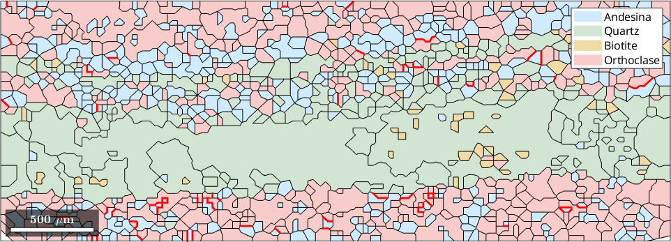
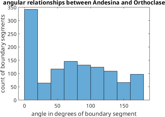
We can also represent the angular misorientation data between these two phases as a histogram.
figure;histogram(angle./degree)
xlabel('angle in degrees of boundary segment')
ylabel('count of boundary segments')
title('angular relationships between Andesina and Orthoclase')