Visualizing ODFs

Since an orientation density function (ODF) is a function on the three dimensional, non Euclidean orientation space its proper visualization is a challenging task. In general one distinguishes two approaches

In order to demonstrate the different visualization techniques let us first define a model ODF.

cs = crystalSymmetry('32');
mod1 = orientation.byEuler(90*degree,40*degree,110*degree,'ZYZ',cs);
mod2 = orientation.byEuler(50*degree,30*degree,-30*degree,'ZYZ',cs);

odf = 0.1*unimodalODF(mod1) ...
  + 0.2*unimodalODF(mod2) ...
  + 0.7*fibreODF(Miller(0,0,1,cs),vector3d(1,0,0),'halfwidth',10*degree);

and lets switch to the LaboTex colormap

setMTEXpref('defaultColorMap',LaboTeXColorMap);

Three Dimensional Plots

Visualizing an ODF in three dimensions is done by the command plot3d.

plot3d(odf)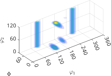

By default this command represents the ODF in the Bunge Euler angle space \(\varphi_1\), \(\Phi\), \(\varphi_2\). The range of the Euler angles depends on the crystal symmetry according to the following table

Note that for the last to symmetries the three fold axis is not taken into account, i.e., each orientation appears three times within the Euler angle region. The first Euler angle is not restricted by any crystal symmetry, but only by specimen symmetry. For an arbitrary symmetry the bounds of the fundamental region can be computed by the command fundamentalRegionEuler

[maxphi1,maxPhi,maxphi2] = fundamentalRegionEuler(crystalSymmetry('432'),specimenSymmetry('222'))

maxphi1 =
    1.5708
maxPhi =
    1.5708
maxphi2 =
    1.5708

This return the common \(90^{\circ} \times 90^{\circ} \times 90^{\circ}\) cube for cubic crystal and orthorombic specimen symmetry. For an arbitrary orientation

ori = orientation.rand(crystalSymmetry('432'),specimenSymmetry('222'))

ori = orientation (432 → xyz (222))
 
  Bunge Euler angles in degree
     phi1     Phi    phi2
  318.657 109.602 155.522

the symmetrically equivalent orientation within the fundamental region can be computed using the command project2EulerFR

[phi1,Phi,phi2] = ori.project2EulerFR;
[phi1,Phi,phi2] ./degree

ans =
   41.3431   70.3981   65.5215

A big disadvantage of the Euler angle representation of the orientation space is that it very badly follows the curved geometry of the space.

Especially for misorientation distribution functions a better alternativ is the three dimensional axis angle space. To visualize an ODF with respect to this parameterization simply add the option 'axisAngle'

plot3d(odf,'axisAngle','figSize','large')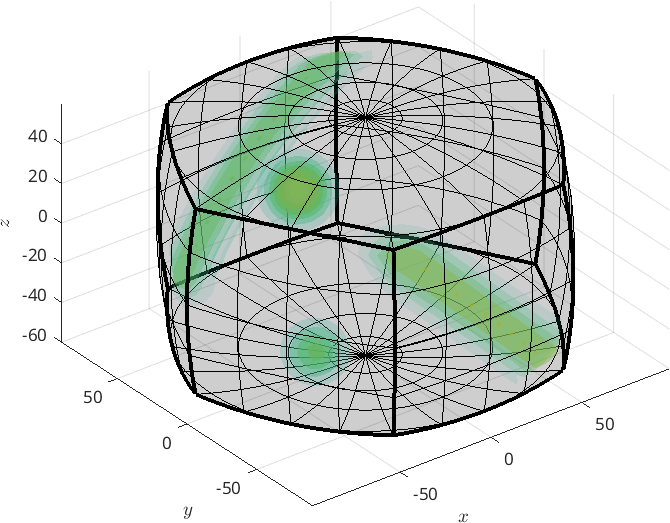

ODF Sections

Plotting an ODF in two dimensional sections through the orientation space is done using the command plotSection. By default the sections are at constant angles of \(\varphi_2\).

plotSection(odf)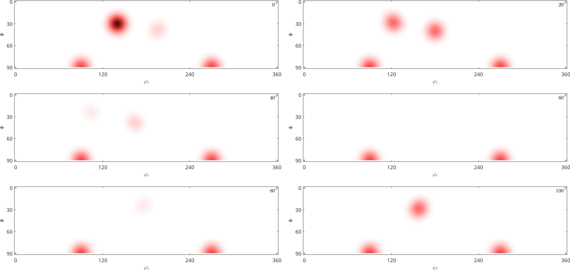

More information how to customize such plots can be found in the chapter Euler angle sections. Beside the standard \(\varphi_2\) sections MTEX supports also sections according to all other Euler angles.

In fact MTEX highly recommends the so called sigma sections as they provide a much less distorted representation of the orientation space. A detailed description of the sigma sections can be found in the chaper sigma sections.

plotSection(odf,'sigma')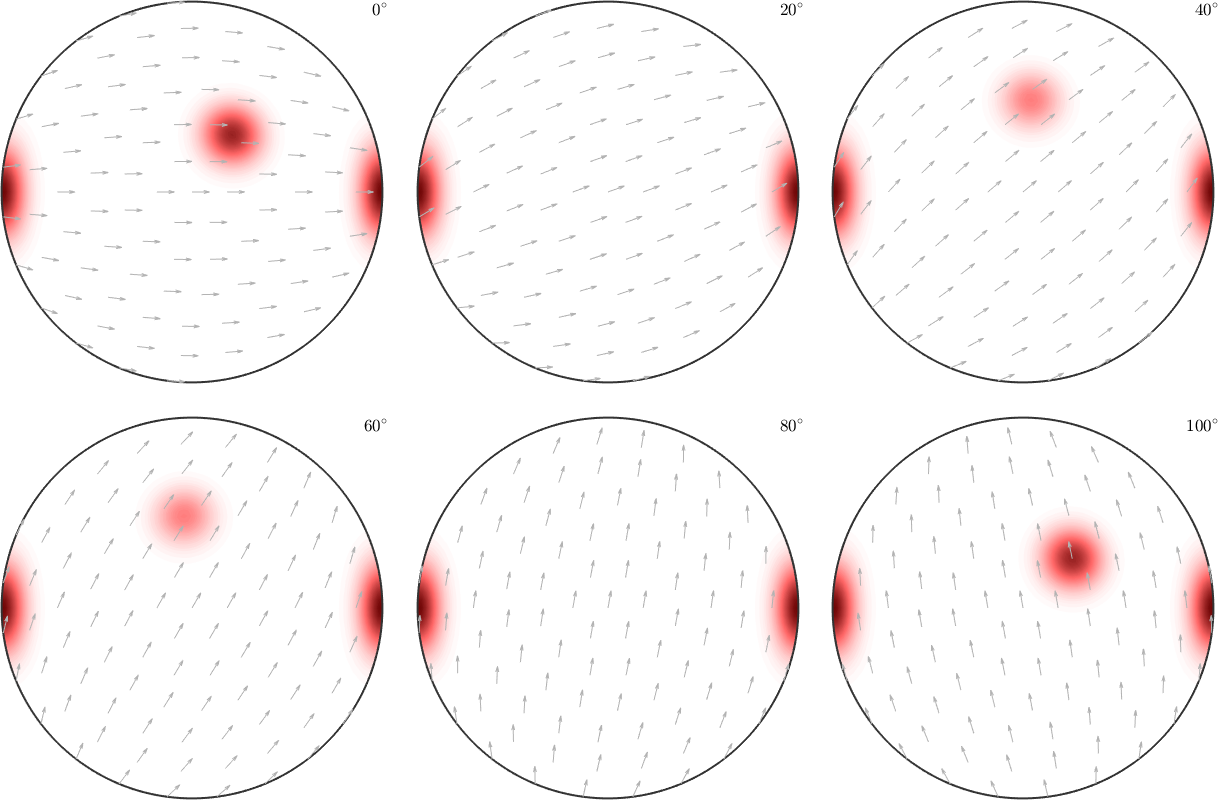

Plotting the ODF along a fibre

For plotting the ODF along a certain fibre we have the command

close all

% select a fibre of interest
f = fibre(Miller(1,2,-3,2,cs),vector3d(2,1,1));

plot(odf,f,'LineWidth',2);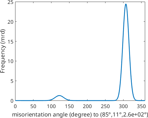

Finally, lets set back the default colormap.

setMTEXpref('defaultColorMap',WhiteJetColorMap);