The Crystal Reference System

The Crystal Reference System edit page

Commonly the crystal coordinate system is defined by the crystallographic axes \(\vec a\), \(\vec b\), \(\vec c\), The length [a,b,c] and the angles [alpha,beta,gamma] between theses axes needs to be specified when defining a variable of type crystalSymmetry.

cs = crystalSymmetry('triclinic',[1,2.2,3.1],[80*degree,85*degree,95*degree])

cs = crystalSymmetry
 
  symmetry          : -1           
  elements          : 2            
  a, b, c           : 1, 2.2, 3.1  
  alpha, beta, gamma: 80°, 85°, 95°
  reference frame   : X||a*, Z||c

Need of a Euclidean reference system

However, there are many crystal properties, like orientation or tensorial properties, that are described with respect to an Euclidean reference system \(\vec x\), \(\vec y\), \(\vec z\) as opposed to the crystallographic axes \(\vec a\), \(\vec b\)s, \(\vec c\). Most importantly, Euler angles describe orientations as subsequent rotations about the \(\vec z\), \(\vec x\) and \(\vec z\) axis. Hence, we need to inscribe an Euclidean reference system \(\vec x\), \(\vec y\), \(\vec z\) into the crystallographic reference system \(\vec a\), \(\vec b\), \(\vec c\).

Note, that also the alignment of the crystal axes \(\vec a\), \(\vec b\) and \(\vec c\) with respect to the atomic lattice, and hence it symmetries, follows different conventions. These are discussed in the section Alignment of the Crystal Axes.

Cubic, tetragona and orthorhombic symmetries

In orthorhombic, tetragonal and cubic crystal symmetry the crystal reference system \(\vec a\), \(\vec b\), \(\vec c\) is itself an Euclidean one and, hence, setting \(\vec x\) parallel to \(\vec a\), \(\vec y\) parallel to \(\vec b\) and \(\vec z\) parallel to \(\vec c\) is a canonical choice.

As for such symmetries this is also the default in MTEX there is no need to specify the alignment seperately.

Trigonal and hexagonal materials

For trigonal and hexagonal materials the z axis is commonly aligned with the \(\vec c\) axis. As for the \(\vec x\) and \(\vec y\) axes they are either aligned with the \(\vec a\) or \(\vec b\) axes.

The following command aligns the \(\vec x\) axes to the \(\vec a\) axes and the \(\vec z\) axes to the \(\vec c\) axes.

cs_x2a = crystalSymmetry('321',[1.7,1.7,1.4],'X||a','Z||c');

% visualize the results
plot(cs_x2a,'figSize','small')
annotate(cs_x2a.aAxis,'MarkerFaceColor','r','label','a','backgroundColor','w')
annotate(cs_x2a.bAxis,'MarkerFaceColor','r','label','b','backgroundColor','w')
annotate(-vector3d.Y,'MarkerFaceColor','green','label','-y','backgroundColor','w')
annotate(-vector3d.X,'MarkerFaceColor','green','label','-x','backgroundColor','w')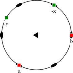

In contrast the following command aligns the \(\vec y\) axes to the \(\vec a\) axes and the \(\vec z\) axes to the \(\vec c\) axes.

cs_y2a = crystalSymmetry('321',[1.7,1.7,1.4],'y||a','Z||c');
plot(cs_y2a,'figSize','small')
annotate(cs_y2a.aAxis,'MarkerFaceColor','r','label','a','backgroundColor','w')
annotate(cs_y2a.bAxis,'MarkerFaceColor','r','label','b','backgroundColor','w')
annotate(-vector3d.Y,'MarkerFaceColor','green','label','-y','backgroundColor','w')
annotate(-vector3d.X,'MarkerFaceColor','green','label','-x','backgroundColor','w')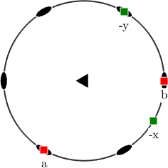

The only difference between the above two plots is the position of the \(\vec x\) and \(\vec y\) axes. The reason is that visualizations relative to the crystal reference system, e.g., inverse pole figures, are in MTEX aligned on the screen according to the b-axis.

This on-screen alignment can be easily modified by

% change on screen alignment
plota2east

% redo last plot
plot(cs_y2a,'figSize','small')
annotate(cs_y2a.aAxis,'MarkerFaceColor','r','label','a','backgroundColor','w')
annotate(cs_y2a.bAxis,'MarkerFaceColor','r','label','b','backgroundColor','w')
annotate(-vector3d.Y,'MarkerFaceColor','green','label','-y','backgroundColor','w')
annotate(-vector3d.X,'MarkerFaceColor','green','label','-x','backgroundColor','w')

% set old default back
plotb2east

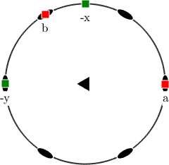
It should be stressed that the alignment between the Euclidean crystal axes \(\vec x\), \(\vec y\), \(\vec z\) and the crystallographic axes \(\vec a\), \(\vec b\) and \(\vec c\) is crucial for many computations. The difference between both setups becomes more visible if we plot crystal shapes in the \(\vec x\), \(\vec y\), \(\vec z\) coordinate system

cS_x2a = crystalShape.quartz(cs_x2a);

close all
figure(1)
plot(cS_x2a,'figSize','small')
hold on
arrow3d(0.5*[xvector,yvector,zvector],'labeled')
hold off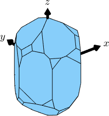

cS_y2a = crystalShape.quartz(cs_y2a);

figure(2)
plot(cS_y2a,'figSize','small')
hold on
arrow3d(0.5*[xvector,yvector,zvector],'labeled')
hold off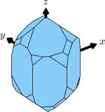

Most important is the difference if Euler angles are used to describe orientation. Lets consider the following two orientations

ori_x2a = orientation.byEuler(0,0,0,cs_x2a)
ori_y2a = orientation.byEuler(0,0,0,cs_y2a)

ori_x2a = orientation (321 → xyz)
 
  Bunge Euler angles in degree
  phi1  Phi phi2
     0    0    0
 
 
ori_y2a = orientation (321 → xyz)
 
  Bunge Euler angles in degree
  phi1  Phi phi2
     0    0    0

and visualize them in a pole figure.

newMtexFigure('innerPlotSpacing',20,'figSize','small')
plotPDF(ori_x2a,Miller(1,0,0,cs_x2a),'MarkerSize',20)
annotate([xvector,yvector],'label',{'x','y'},'backgroundColor','w')
nextAxis
plotPDF(ori_y2a,Miller(1,0,0,cs_y2a),'MarkerSize',20)
annotate([xvector,yvector],'label',{'x','y'},'backgroundColor','w')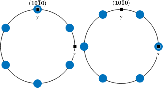

We observe that both pole figures are rotated with respect to each other by 30 degree. Indeed computing the misorientation angle between both orientations gives us

angle(ori_x2a, ori_y2a) ./ degree

The involved symmetries have different reference systems
  1: 321, X||b*, Y||a, Z||c
  2: 321, X||a, Y||b*, Z||c*
  I'm going to transform the data from the first one to the second one
 
ans =
   30.0000

In many cases MTEX automatically recognizes different setups and corrects for this. In order to manually transform orientations or tensors from one reference frame into another reference frame one might use the command transformReferenceFrame. The following command transforms the reference frame of orientation ori_y2a into the reference frame cs_x2a

ori_x2a.transformReferenceFrame(cs_y2a)

ans = orientation (321 → xyz)
 
  Bunge Euler angles in degree
  phi1  Phi phi2
   270    0    0

Triclinic and monoclinic symmetries

In triclinic and monoclinic symmetries even more different setups are used. As two perpendicular crystal axes are required to align with \(\vec x\), \(\vec y\) or \(\vec z\) one usually chooses one crystal axis from the direct coordinate system, i.e., \(\vec a\), \(\vec b\) or \(\vec c\), and the second crystal axis from the reciprocal axes \(\vec a^*\), \(\vec b^*\) or \(\vec c^*\). Typical examples for such setups are

cs = crystalSymmetry('-1', [8.290 12.966 7.151], [91.18 116.31 90.14]*degree,...
  'x||a*','y||b', 'mineral','An0 Albite 2016')

cs = crystalSymmetry
 
  mineral           : An0 Albite 2016        
  symmetry          : -1                     
  elements          : 2                      
  a, b, c           : 8.3, 13, 7.2           
  alpha, beta, gamma: 91.18°, 116.31°, 90.14°
  reference frame   : X||a*, Y||b

cs = crystalSymmetry('-1', [8.290 12.966 7.151], [91.18 116.31 90.14]*degree,...
  'x||a','c||c*', 'mineral','An0 Albite 2016')

%
%
%<html>
%   <div class="note">
%      <b>ok&lt;*NASGU&gt;
%</b>
%      <text/>
%   </div>
%</html>
%

cs = crystalSymmetry
 
  mineral           : An0 Albite 2016        
  symmetry          : -1                     
  elements          : 2                      
  a, b, c           : 8.3, 13, 7.2           
  alpha, beta, gamma: 91.18°, 116.31°, 90.14°
  reference frame   : X||a, Z||c*