Select Grain Boundaries

A grain boundary is stored as a list of short segments. Each segment lies between two neighbouring measurements that belong to different grains. Selecting boundaries therefore means indexing this list, and every selection returns another grainBoundary list.

This page assumes that the map has already been divided into grains as in Grain Reconstruction. The Grain Boundaries overview explains how these segments represent an interface in a two-dimensional section.

close all;

% import the data
plottingConvention.default('y↑→x');
mtexdata forsterite silent

% restrict it to a subregion of interest
ebsd = ebsd(inpolygon(ebsd,[5 2 10 5]*10^3));

% reconstruct and smooth the grains
[grains,ebsd] = calcGrains(ebsd,'minPixel',5,'alpha',10);
grains = smoothBoundary(grains,4);

% extract and plot the complete boundary list
gB = grains.boundary;
plot(ebsd)
hold on
plot(gB,'lineWidth',2)
hold off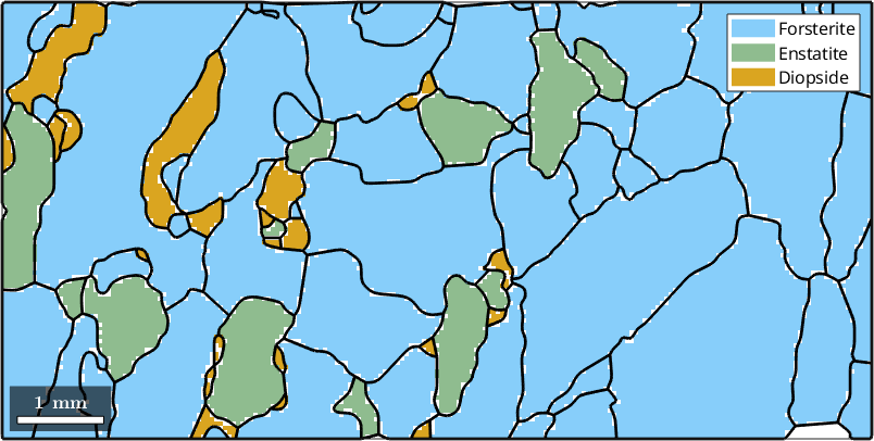

The black network contains every boundary segment in the cropped map. It includes boundaries between grains of one phase, boundaries between phases, and the outer rim of the scan.

What the list contains

Displaying gB reports the number and total length of the segments for every pair of phases that meets in the map.

gB

gB = grainBoundary (y↑→x)
 
 Segments    length   mineral 1   mineral 2
      555  27532 µm  notIndexed  Forsterite
       32   1586 µm  notIndexed   Enstatite
       29   1386 µm  notIndexed    Diopside
     1178  54925 µm  Forsterite  Forsterite
      554  26047 µm  Forsterite   Enstatite
      440  20260 µm  Forsterite    Diopside
       27   1278 µm   Enstatite   Enstatite
      123   5723 µm   Enstatite    Diopside
       22    930 µm    Diopside    Diopside

The rows involving notIndexed combine two situations. Some segments border a connected notIndexed area, whose diffraction patterns could not be indexed. Others lie on the outer rim, where a grain is cut off by the scan and has no neighbour on the other side. Selecting Grains shows how to identify grains at that rim.

By the phases on either side

Two phase names select segments between those phases. The first selection contains forsterite to forsterite boundaries, which separate differently oriented grains of the dominant phase.

gB_FoFo = gB('Fo','Fo');

plot(ebsd)
hold on
plot(gB_FoFo,'lineColor','blue','micronbar','off','lineWidth',4)
hold off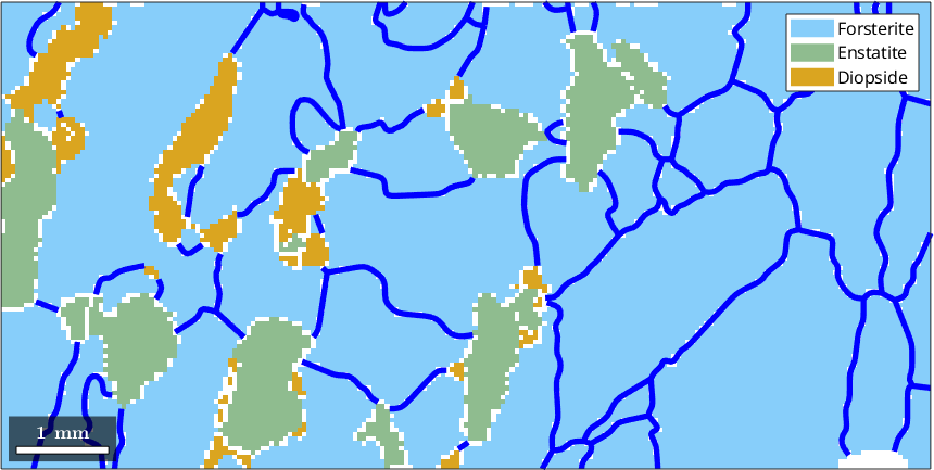

The thick blue segments occur within the forsterite part of the phase map. They do not include its contacts with the other minerals.

The next selection contains forsterite to enstatite boundaries. A phase boundary is not a separate object in MTEX. It is a grain boundary whose two neighbouring grains happen to differ in phase.

gB_FoEn = gB('Fo','En');

plot(ebsd)
hold on
plot(gB_FoEn,'lineColor','darkgreen','micronbar','off','lineWidth',4)
hold off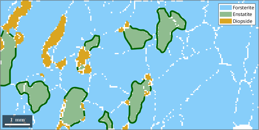

The green segments follow only contacts between the forsterite and enstatite regions. They are two different crystals meeting, rather than two orientations of the same phase.

Why phase order matters

The order of the phase names matters for more than readability. A misorientation is a rotation from one crystal to another, so reversing the names gives inverse misorientations. A misorientation axis expressed in crystal coordinates therefore refers to whichever crystal was named first.

mori = gB('Fo','En').misorientation(1)

inv(mori)

mori = misorientation (Forsterite → Enstatite)
 
  Bunge Euler angles in degree
     phi1     Phi    phi2
  239.134 51.5067 125.138
 
 
ans = misorientation (Enstatite → Forsterite)
 
  Bunge Euler angles in degree
     phi1     Phi    phi2
  54.8624 51.5067 300.866

The two phase orders select the same physical segments, but reversing the sides also reverses the walk along every boundary chain. The segments are consequently not returned in the same row order. Corresponding segments have exactly inverse misorientations, but gB('En','Fo').misorientation(1) is a different segment from the first one selected above.

By grain

A boundary list is also available from the grains it belongs to. This is how to ask for the boundary of one grain or of a grain selection. Here grains(47) means the 47th grain in the current list, not necessarily a grain whose ID is 47; Selecting Grains explains the distinction between list position and grain ID.

grains(47).boundary

plot(ebsd)
hold on
plot(grains(47).boundary,'lineWidth',4,'lineColor','DarkBlue')
hold off

ans = grainBoundary (y↑→x)
 
 Segments   length   mineral 1  mineral 2
       23  1077 µm  Forsterite   Diopside
        7   311 µm   Enstatite   Diopside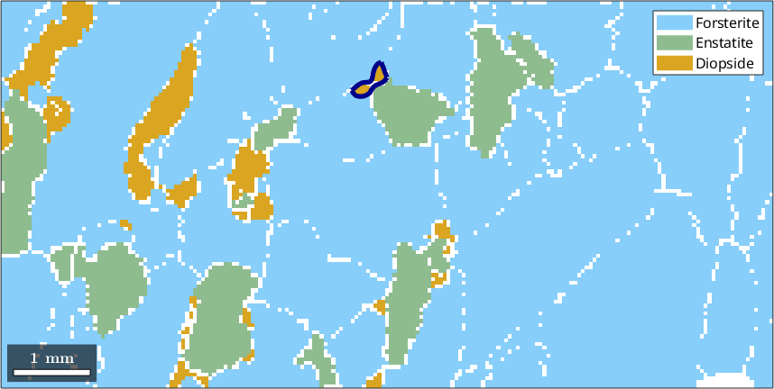

The dark-blue outline includes every phase pair on the boundary of this grain. The displayed boundary summary names the phases on its far side.

Boundaries inside a grain

grains.innerBoundary stores segments between two measurements of the same grain. They arise when the segmentation criterion separates two neighbouring pixels, but another path through the map still connects them into one phase-homogeneous grain. An orientation gradient that comes back around can produce exactly this situation.

grains.innerBoundary

plot(ebsd)
hold on
plot(grains.innerBoundary,'lineColor','red','lineWidth',4)
hold off

ans = grainBoundary (y↑→x)
 
 Segments  length   mineral 1   mineral 2
       11  482 µm  Forsterite  Forsterite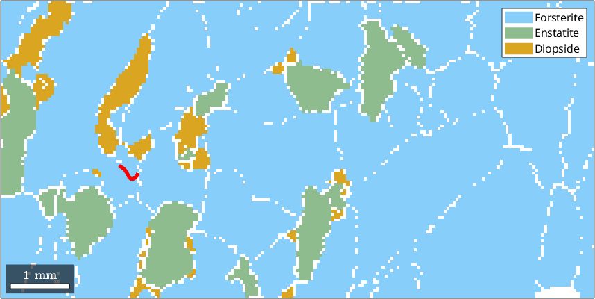

The display reports 11 inner-boundary segments in this barely deformed rock. The red segments sit inside connected grains rather than tracing complete grain outlines. Deformed material may contain many more, and Subgrain Boundaries explains how a two-threshold reconstruction preserves a systematic low-angle population.

By misorientation or another property

Every segment carries its misorientation. A logical condition on the misorientation angle therefore selects segments in the same way as any MATLAB logical index. Here the eligible set is first restricted to forsterite to forsterite boundaries, so every angle has one consistent pair of crystal symmetries.

isHighAngle = gB_FoFo.misorientation.angle > 60*degree;
gB_high = gB_FoFo(isHighAngle)

plot(ebsd)
hold on
plot(gB_FoFo,'lineColor','lightgray','lineWidth',2)
plot(gB_high,'lineColor','red','lineWidth',4)
hold off

gB_high = grainBoundary (y↑→x)
 
 Segments    length   mineral 1   mineral 2
      478  22160 µm  Forsterite  Forsterite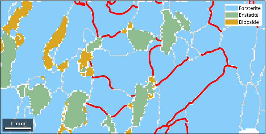

The grey segments are all eligible forsterite boundaries, while red marks only those above the chosen angle. The same pattern works with a condition on position, direction, length, or any other per-segment property; see Grain Boundary Properties.

More specialised misorientation selections compare an axis, a complete rotation, or a coincidence site lattice relationship. They are developed in Twist and Tilt, Twinning, and CSL.

Next

Boundary Plots shows how to colour the selected segments by scalar, directional, and full-misorientation data. Grain Boundary Properties then develops the per-segment values from which more selections can be built.

Further reading