Properties of Three-Dimensional Grains

Three dimensional grain share many of the properties of two dimensional grains, e.g. grains.meanOrientation. However, the geometric properties are quite different. These are

We start our discussion by importing some sample data set of three dimensional grains

mtexdata NeperGrain3d

plot(grains,grains.meanOrientation,'micronbar','off')

% set camera
setCamera(plottingConvention.default3D)

grains = grain3d
 
 Phase  Grains   Volume  Mineral  Symmetry  Crystal reference frame
     2    1000  1000000   Quartz       321       X||a*, Y||b, Z||c*
 
 boundary faces: 7203
 
 Properties: meanRotation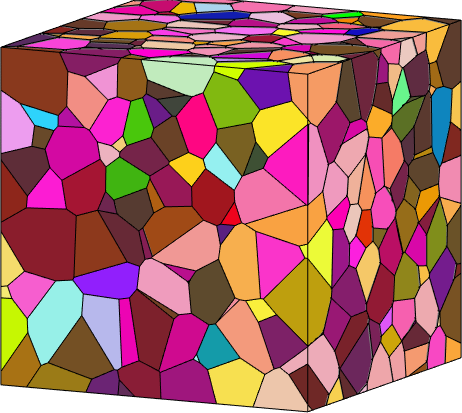

Grain volume

The most basic properties are diameter, surface and volume. Those can be computed by

grains(9).diameter

ans =
   19.4556

grains(9).surface

ans =
  765.9084

grains(9).volume

ans =
   1.4318e+03

The units are µm, µm² and µm³. We may analyze the distribution of grains by grain volume using a histogram.

close all
histogram(grains.volume,20,'FaceColor',grains.color)
xlabel('grain volume in µm³')
ylabel('number of grains')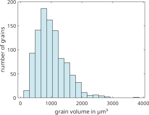

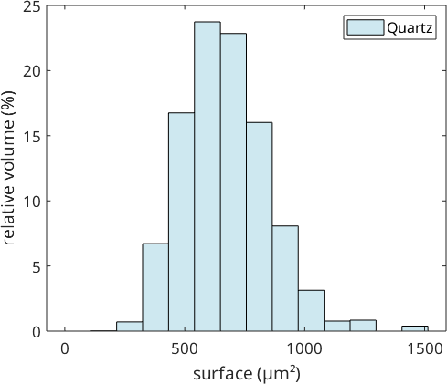
Note that in the above histogram all grains contribute equally independently of their size. We obtain a more realistic histogram if we do not plot the number of grains at the y-axis but its total volume. This can be achieved with the command histogram(grains).

histogram(grains,20)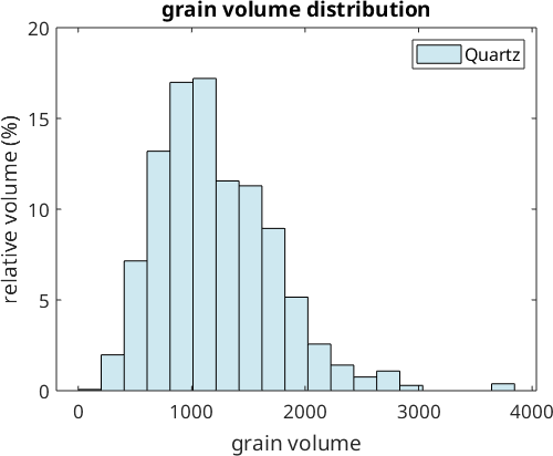

Similarly, we can visualize the distribution of surface or diameter with respect to grain volume or number of grains.

histogram(grains.surface,'FaceColor',grains.color)
xlabel('surface (µm²)')
ylabel('number of grains')

figure
histogram(grains,grains.surface)
xlabel('surface (µm²)')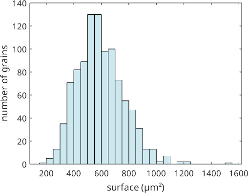

We may also investigate the correlation between any properties using a scatter plot. Almost surely, we find a relationship between the grain diameter and the volume.

scatter(grains.volume.^(1/3), grains.diameter)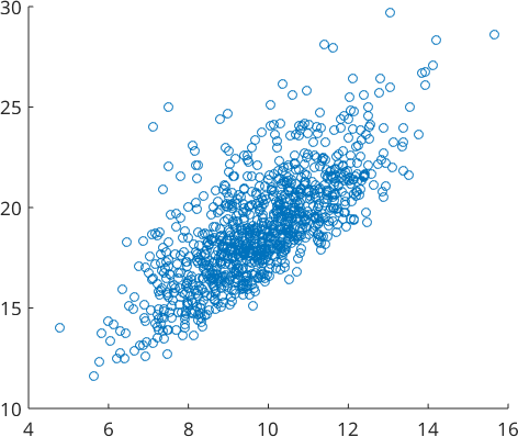

Ellipsoid Based Properties

Similarly as for two dimensional grains the command principalComponents computes the principle axes a, b and c of each grain. These can be interpreted as the half-axes of an ellipsoid fitted to the grain.

[a,b,c] = principalComponents(grains);

Lets use these half-axes to visualize the 3d-grains as ellipsoids colorized by the grain orientation. This is done using the command plotEllipsoid

% compute the color for each ellipsoid
cKey = ipfColorKey(grains.CS);
color = cKey.orientation2color(grains.meanOrientation);

plotEllipsoid(grains.centroid,a,b,c,'faceColor',color);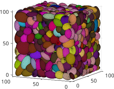

Vertices, grain and surface centroids

Each grain has a set of vertices grains.V and a centroid grains.centroid. Furthermore, each grain boundary element has a centroid. Lets visualize those quantities.

close all
plot(grains(5),'FaceAlpha',0.5,'linewidth',2)

hold on
plot(grains(5).centroid)
plot(grains(5).V)
plot(grains(5).boundary.centroid)
hold off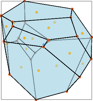

Grain boundary properties

The grain boundary elements the have the following geometric properties

Let us first visualize the grain boundary normals

hold on
quiver(grains(5).boundary,grains(5).boundary.N,'antipodal','linewidth',2)
hold off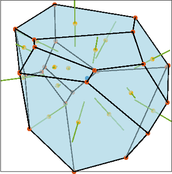

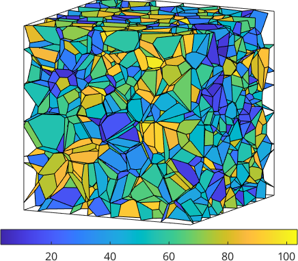
In the next plot we colorize the boundary planes by the misorientation angle of the neighbouring grains.

close all
plot(grains.boundary('indexed'),...
  grains.boundary('indexed').misorientation.angle./degree,'micronbar','off')

setCamera(plottingConvention.default3D)
colorbar('location','southoutside')