Texture evolution in rolled magnesium during uniaxial tension

Texture evolution in rolled magnesium during uniaxial tension edit page

This examples models the texture evolution of rolled magnesium under unixaxial tension using the Taylor model. The undeformed material is assumed to have a basal fibre texture perpendicular to tension direction. Then tension experiment has been performed twice: at room temperature and at 250 degree Celcius. The strain at fracture was approx. 30 percent and 70 percent, respectively.

Setting up hexagonal crystal symmetry

First we need to set up hexagonal crystal symmetry.

cs = crystalSymmetry.load('Mg-Magnesium.cif')
cs = cs.properGroup;

cs = crystalSymmetry
 
  mineral        : Mg                
  symmetry       : 6/mmm             
  elements       : 24                
  a, b, c        : 3.2, 3.2, 5.2     
  reference frame: X||a*, Y||b, Z||c*

Setting up the basal fibre texture

Second, we set up the initial fibre texture which has the c-axis perpendicular to the (x,y)-sheet plane and the a-axes are randomized. This is typical for rolled Mg-sheet

odf = fibreODF(cs.cAxis, vector3d.Z);
%odf = uniformODF(cs)

Plot polefigures of generated initial state without strains

define crystal orientations of interest for polefigures and plot figure

h = Miller({0,0,0,1},{1,0,-1,0},{1,0,-1,1},cs);

pfAnnotations = @(varargin) text([-vector3d.X,vector3d.Y],{'Tension','TD'},...
  'BackgroundColor','w','tag','axesLabels',varargin{:});
setMTEXpref('pfAnnotations',pfAnnotations);
plotPDF(odf,h,'antipodal','contourf','figSize','small')
mtexColorbar;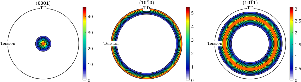

Setting up the slip systems

The critical resolved shear stresses (CRSS) needed to activate certain slip systems is temperature AND material dependant. As it is not trivial to measure/define CRSS, there are many different values in literature.

In practise, at room temperature basal slip dominates and commonly simple tension twins are activated as well (they have very low CRSS). During tension stress perpendicular to the c-axis tension twinning cannot occur. Thats why it is sensible to only define compression twins (which in Mg have a very high CRSS)

% second argument is CRSS normalized to basal slip
sScold = [slipSystem.basal(cs,1),...
  slipSystem.prismatic2A(cs,66),...
  slipSystem.pyramidalCA(cs,80),...
  slipSystem.twinC1(cs,100)];

% consider all symmetrically equivlent slip systems
[sScold,slipId] = sScold.symmetrise;

At higher temperatures the CRSS of non-basal slip systems decreases.

% second argument is CRSS normalized to basal slip
sSwarm = [slipSystem.basal(cs,1),...
  slipSystem.prismatic2A(cs,15),...
  slipSystem.pyramidalCA(cs,10),...
  slipSystem.twinC1(cs,100)];

% consider all symmetrically equivlent slip systems
sSwarm = sSwarm.symmetrise;

Defining strain tensors

Due to constant volume law, the sum of all strains must equal zero. Here slightly anisotropic strain is assumed at room temperature, with more thinning in y-direction than in z-direction. In practise the anisotropy of Mg at high temperatures becomes negligible.

epsCold = 0.3 * strainTensor(diag([1 -0.6 -0.4]))
epsWarm = 0.7 * strainTensor(diag([1 -0.5 -0.5]))

epsCold = strainTensor (xyz)
  type: Lagrange 
  rank: 2 (3 x 3)
 
 *10^-2
  30   0   0
   0 -18   0
   0   0 -12
 
epsWarm = strainTensor (xyz)
  type: Lagrange 
  rank: 2 (3 x 3)
 
 *10^-2
  70   0   0
   0 -35   0
   0   0 -35

Calculate texture evolution

The Tayor calculation is used to get the resulting spin of each vector as well as the coeffeicients for each slip system for cold and hot state

% simulated an initial orientation distribution of 10000 grains
ori = odf.discreteSample(100000);

% apply the Taylor model
[~,bCold,WcoldD] = calcTaylor( inv(ori) .* epsCold, sScold);
[~,bWarm,WwarmD] = calcTaylor( inv(ori) .* epsWarm, sSwarm);

Apply the Taylor spin to the initial orientation distribution

oriCold = ori .* orientation(-WcoldD);
oriWarm = ori .* orientation(-WwarmD);

nextAxis %create a new axis on the existing figure and put along side
plotPDF(oriCold,h,'antipodal','contourf','grid','grid_res',30*degree)
mtexColorbar;

nextAxis %create a new axis on the existing figure and put along side
plotPDF(oriWarm,h,'antipodal','contourf','grid','grid_res',30*degree)
mtexColorbar;

% get figure handle and set correct layout
mtexFig = gcm;
mtexFig.ncols = 3; mtexFig.nrows = 3; mtexFig.layoutMode = 'user';
drawNow(gcm)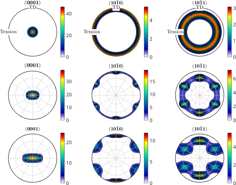

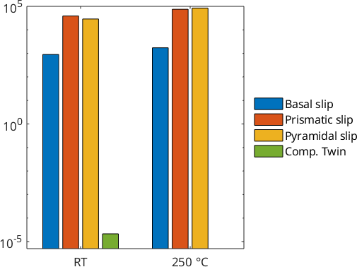
Statistics on activated slip systems

By adding up the coefficients of the taylor calculation and grouping them according to their slip system type, a bar chart can be plotted

% ensure slipId has the same size as |bCold|
slipId = repmat(slipId.',length(ori),1);

% sum up the sliprates of symmetrically equivalent slip systems, i.e.,
% those that have the same |slipId|
statSsCold = accumarray(slipId(:),bCold(:));
statSsWarm = accumarray(slipId(:),bWarm(:));

The results can be plotted with logarithmic scale for better visualization

figure(2)
bar([statSsCold.';statSsWarm.'])
set(gca, 'YScale', 'log','XTickLabel', {'RT' '250 °C'})
legend({'Basal slip','Prismatic slip','Pyramidal slip','Comp. Twin'},...
    'Location','eastoutside')
legend('boxoff')