Orientation Sections

Why Section Plots

A three-dimensional cloud of orientations is hard to read on paper. A section plot replaces it with a stack of two-dimensional slices through orientation space. The choice of slices is a convention: each one keeps some structure recognisable and hides something else.

This page assumes the crystal-to-specimen map from Theory, the symmetry-equivalent representatives from Symmetry, and the rotation coordinates from Rotation Representations. 3D Plots shows the spaces that are cut here.

A reference frame is the coordinate system in which data are expressed. A plotting convention states how that frame is laid out on screen. The convention below draws specimen Y upward and specimen X to the right. It does not rotate the orientations or change their reference frames.

plottingConvention.default('y↑→x');

cs = crystalSymmetry('432');
ss = specimenSymmetry('222');

ori = orientation.rand(100,cs,ss);

How a Point Enters a Section

A mathematical slice has zero thickness, so a finite random sample would almost never land on one exactly. plotSection therefore draws an orientation when its section coordinate lies within a tolerance of the panel value. The 'tolerance' option sets this half-width; its default is \(5^\circ\), and MTEX narrows it when the requested panels are closer together.

These tolerance bands are not an exhaustive partition of the input. An orientation may miss every panel. In Euler and sigma sections, MTEX also tests proper symmetry-equivalent representatives, so one input orientation may give more than one visible point. Axis--angle sections instead place one symmetry-reduced representative in the fundamental region.

phi2 Sections

The classical cut fixes the third Bunge Euler angle \(\varphi_2\). Each panel is labelled by its value of \(\varphi_2\), while \(\varphi_1\) and \(\Phi\) span the rectangular plane.

plotSection(ori,'phi2')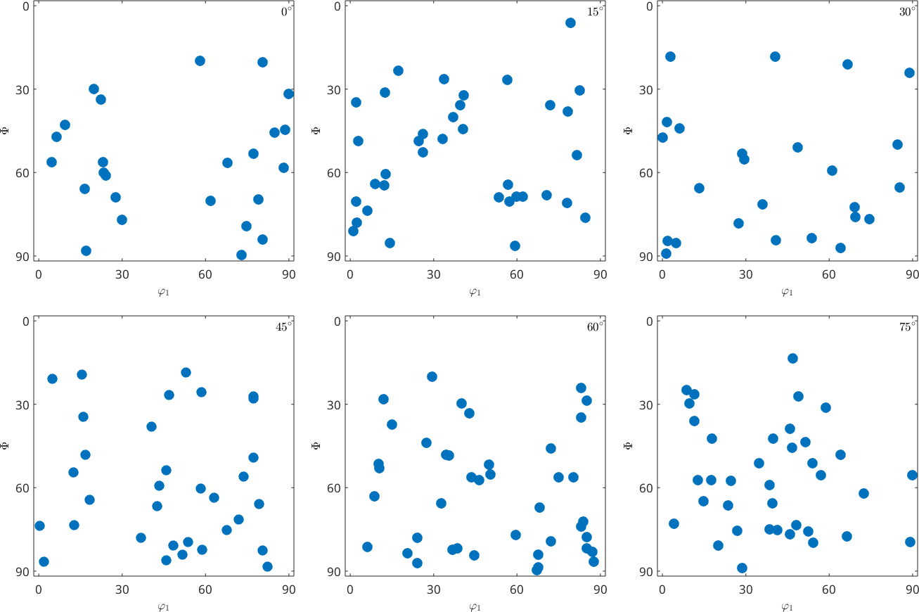

The points have no preferred orientation, but they are not uniform in these rectangular coordinates. The orientation-space volume element contains \(\sin\Phi\), so the cloud thins towards \(\Phi=0\) at the top of each panel. This is the baseline expected from a uniform orientation distribution, not evidence for a texture.

A real texture adds spots or lines that continue through several panels. The classical rolling fibres of cubic metals are commonly read this way; see Euler Angle Sections.

Sigma Sections

Sigma sections reorganise the same three orientation coordinates around a selected crystal axis. MTEX uses the Matthies coordinate \(\sigma=\alpha+\gamma\). Do not identify it with the informal Bunge-angle expression \(\sigma=\varphi_1-\varphi_2\) sometimes attached to these plots; that is not the coordinate computed here.

plotSection(ori,'sigma')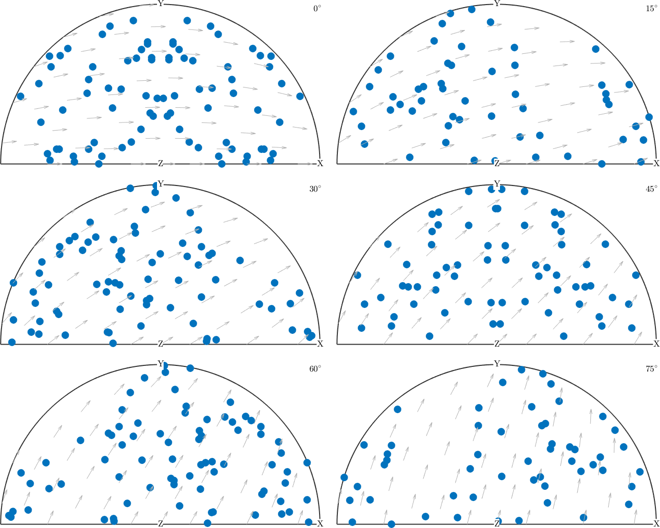

Each half-disc is a pole-figure-like view of the crystal \(c^*\) axis. The grey arrows show the reference direction for the remaining rotation, and that field turns from one panel to the next. Repeated blue points are symmetry-equivalent representatives, not additional input orientations.

Sigma sections can keep a texture component together instead of splitting it across several Euler sections. The rule of thumb that they need fewer panels does not hold for the defaults here: both commands make six. The claim that they are always the better default for cubic material is also too broad. Compare both views for the texture and symmetry at hand. Sigma Sections uses a structured ODF to show when their geometric reading is especially useful.

Axis--Angle Sections

Axis--angle sections fix the rotational angle \(\omega\). A point within a panel gives the corresponding rotation axis. The option 'sections' sets the number of angle bands.

plotSection(ori,'axisAngle','sections',6)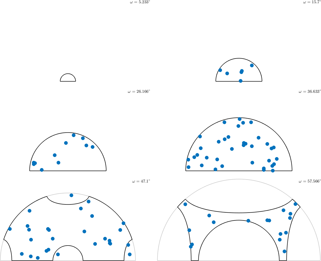

Read the angle above each panel together with its outline. The outline is the allowed axis sector at that angle, and its changing shape is the effect of crystal and specimen symmetry on the fundamental region. MTEX volume-scales these panels by default, so their displayed diameters do not share one angular scale.

Further Section Types

plotSection also accepts 'phi1' and 'Phi' for the other Bunge Euler angles, and 'alpha' or 'gamma' for Matthies Euler angles. The option 'sections' chooses the number of panels. An explicit vector supplied with a section name chooses their values instead.

An orientation distribution function (ODF) is a density on orientation space. The same section geometries can display an ODF, which is their main use in texture analysis; see Plotting an ODF. Do not contour a scatter of orientations directly. Computing an ODF first and plotting that density is both faster and better founded, and MTEX warns when asked to contour the scatter itself.

References

Next

Return to 3D Plots when the connection between a section and its full space is unclear. Continue with Fundamental Regions to understand the symmetry-dependent outlines in the axis--angle panels. The next chapter, Misorientations, makes axis--angle sections a central view of relative orientations.

References

- H.-J. Bunge, Texture Analysis in Materials Science: Mathematical Methods, Butterworths, English ed., 1982, develops Euler orientation space and classical ODF sections.
- S. Matthies, K. Helming, and K. Kunze, On the Representation of Orientation Distributions in Texture Analysis by Sigma-Sections. I. General Properties of Sigma-Sections, physica status solidi (b) 157 (1990), 71-83, introduces the section family and compares its distortions.
- S. Matthies, K. Helming, and K. Kunze, On the Representation of Orientation Distributions in Texture Analysis by Sigma-Sections. II. Consideration of Crystal and Sample Symmetry, Examples, physica status solidi (b) 157 (1990), 489-507, develops the symmetry-dependent regions and their relation to pole and inverse pole figures.