ODF Characteristics

An orientation distribution function (ODF) lives on a three-dimensional space, so no single plot contains all of it. A handful of numbers can say where the texture is strongest, how concentrated it is, and what fraction of the material lies near a chosen component. These are the quantities commonly quoted when textures are compared.

This page assumes the normalization and multiples of a random distribution (mrd) introduced in ODF Theory. The model constructions come from ODF Modeling. Every ODF below has mean 1, so its integrals can be read as material fractions.

plottingConvention.default('y↑→x');

Three ODFs to Measure

The first example is a bimodal ODF. Its two normalized components have equal mixture weights, so the mixture also has mean 1.

cs = crystalSymmetry('mmm');
odfBimodal = 0.5*unimodalODF(orientation.byEuler(0,0,0,cs)) + ...
  0.5*unimodalODF(orientation.byEuler(30*degree,0,0,cs));

The second example is a fibre ODF. It concentrates orientations around the fibre that aligns the crystal direction \((001)\) with specimen X.

f001X = fibre(Miller(0,0,1,cs),vector3d.X);
odfFibre = fibreODF(f001X);

The third example was estimated from neutron pole figures of quartz. The Dubna Example reconstructs it from the measured files. Here the cached reconstruction keeps the focus on its characteristics, while the measured pole-figure directions remain available for the plot below.

mtexdata dubna silent
odfMeasured = mtexdata('dubnaODF');

The Modal Orientation

A mode is a local maximum of the ODF. Its value is a density in mrd, not a percentage of material. max returns the global maximum and the orientation where it is attained.

[peakValue,preferredOrientation] = max(odfMeasured)

peakValue =
   93.9665
 
preferredOrientation = orientation (Quartz → y↑→x)
 
  Bunge Euler angles in degree
    phi1     Phi    phi2
  134.38 35.5039 205.572

The printed peak value is in mrd. The square markers show the poles of its orientation on pole figures calculated from the measured ODF.

plotPDF(odfMeasured,pf.allH,'antipodal','superposition',pf.c);
annotate(preferredOrientation,'marker','s','MarkerFaceColor','black');
mtexColorbar('title','mrd');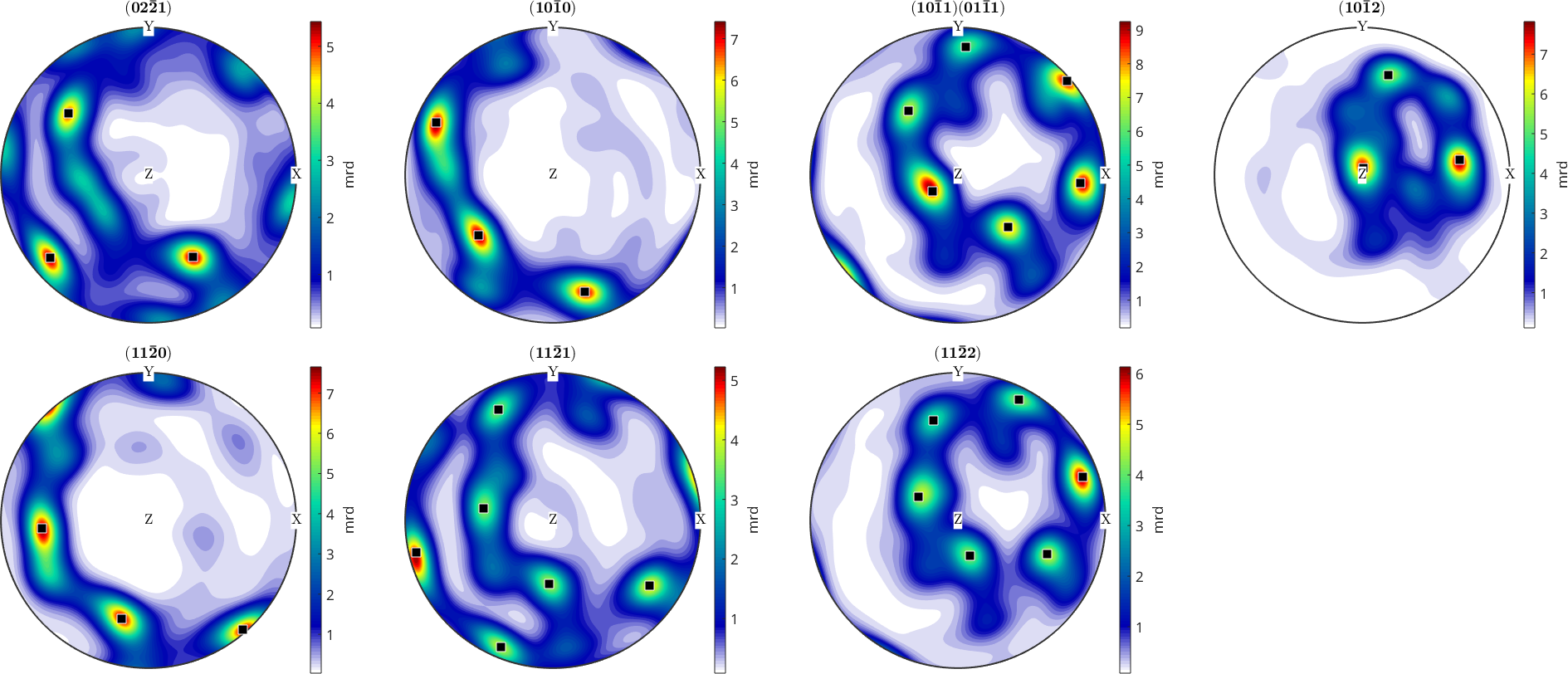

In this example the markers lie in the strongest pole-density regions. That agreement is a useful visual check, but it is not an identity: a pole figure integrates the ODF along fibres, so its maximum need not be the projection of the ODF maximum.

Peak values are especially sensitive to the halfwidth and resolution used to estimate an ODF. Compare them only when those choices are comparable. Density Estimation explains the halfwidth choice. max(odf,'numLocal',n) returns several local modes; Component Analysis explains how to interpret them.

Texture Index

The texture index, also called the J-index, is the mean square of a normalized ODF,

\[ J(f) = \int_{SO(3)} f®^2\,\mathrm{d}R. \]

The orientation-space measure is normalized as in ODF Theory. The index is 1 for a uniform texture and grows without bound as a texture sharpens. A direct numerical integration gives

textureIndexByMean = mean(odfBimodal.*odfBimodal)

textureIndexByMean =
   72.1424

The same quantity is obtained faster and more accurately from harmonic coefficients by squaring the norm.

textureIndexBimodal = norm(odfBimodal)^2

textureIndexBimodal =
   72.1700

The two printed values agree up to the quadrature error of the direct calculation. The measured ODF has a much smaller index, so its texture is much weaker than the model built from two sharp components.

textureIndexMeasured = norm(odfMeasured)^2

textureIndexMeasured =
   16.2135

Entropy

Entropy is another global measure of concentration,

\[ H(f) = -\int_{SO(3)} f®\ln f®\,\mathrm{d}R. \]

It runs in the opposite direction: it is 0 for the uniform ODF and is negative for every nonuniform ODF. A sharper distribution has a more negative entropy.

fibreEntropy = entropy(odfFibre)

fibreEntropy =
   -2.8402

Texture index and entropy both summarize sharpness, but they are not interchangeable. Two ODFs can have the same texture index and different entropies. Like the maximum, both values change when smoothing changes; report the ODF estimation choices with them.

Volume Fractions

A volume fraction asks a more local question: what fraction of the material lies within a chosen disorientation angle of an orientation or a fibre? volume integrates the normalized ODF over either region.

preferredVolumePercent = ...
  100 * volume(odfMeasured,preferredOrientation,30*degree)

preferredVolumePercent =
   37.9843

The printed result is the percentage within \(30^\circ\) of the preferred orientation. Around a fibre, the same command integrates a tube in orientation space.

fibreVolumePercent = 100 * volume(odfFibre,f001X,20*degree)

fibreVolumePercent =
   95.1633

The printed fibre fraction is large because this ODF is the chosen fibre spread with the default halfwidth. Integrated fractions are generally more stable than a peak value when the integration radius is broader than the smoothing scale.

The radius remains part of the result and must be reported. Regions around different components can overlap, so their separately calculated volume fractions need not add to 100 percent. Volume fractions are what turn a density into a statement about the material, as explained in ODF Theory.

References

Next

Locating and partitioning components is Component Analysis; constructing or fitting model components is ODF Modeling. Use Visualizing ODFs when the result should be a plot rather than a number. The next page, Radial ODFs, develops the localized model used in the bimodal example.

References

- H.-J. Bunge, Texture Analysis in Materials Science: Mathematical Methods, Butterworths, English ed., 1982, develops the ODF normalization and texture index.
- R. Hielscher, H. Schaeben, and D. Chateigner, On the Entropy to Texture Index Relationship in Quantitative Texture Analysis, Journal of Applied Crystallography 40 (2007), 371--375, proves bounds between the two measures without making them equivalent.