Line intersections

A straight line drawn across a microstructure is a one-dimensional probe. Every grain boundary it crosses ends one intercept and starts the next. Counting these crossings is one of the oldest measurements in microscopy. On a micrograph it needs neither labelled grain regions nor a model for grain shape, only visible boundaries and a calibrated ruler.

In MTEX the boundary network comes from grain reconstruction. A grain boundary starts as a list of short segments. Each segment lies between neighbouring EBSD pixels assigned to different grains. The intersect command finds where a test line crosses that reconstructed boundary network.

We use a magnesium map containing thin twin lamellae. Smoothing removes the pixel-grid staircase, but it also moves the boundary. Use the same documented smoothing settings when comparing measurements between maps.

plottingConvention.default('y↑→x');
mtexdata twins silent

[grains,ebsd] = calcGrains(ebsd);
grains = grains.smoothBoundary;
gB = grains.boundary;

plot(grains,'FaceColor',[0.8 0.8 0.8])
hold on
plot(gB,'LineWidth',2)
hold off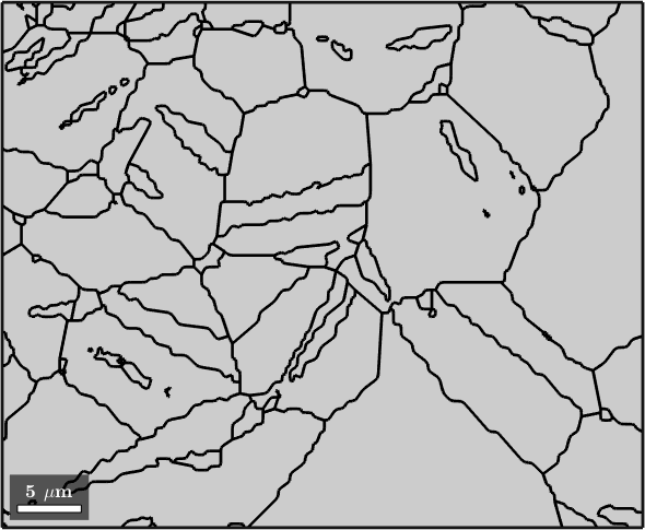

The black network is the smoothed grain boundary. Notice the thin, elongated twin lamellae enclosed by much broader grains.

Define a test line

A line is specified by its start and end points in map coordinates.

xy1 = [10,10]; % start point
xy2 = [41,41]; % end point

hold on
line([xy1(1);xy2(1)],[xy1(2);xy2(2)], ...
  'LineStyle',':','LineWidth',4,'Color','w')
hold off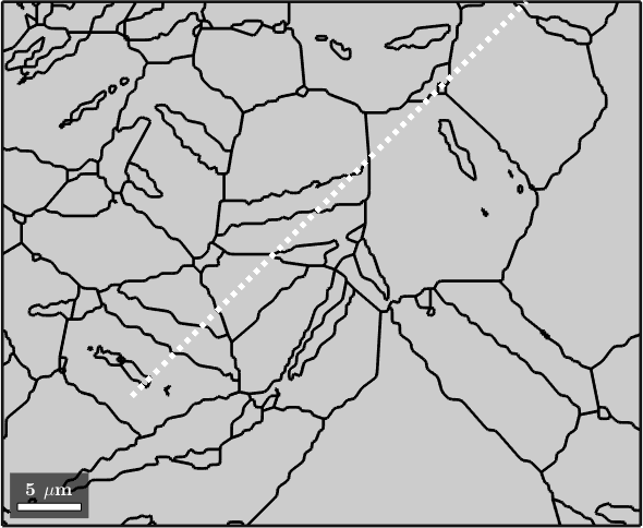

The white diagonal crosses the lamellae obliquely. Its direction is part of the measurement, not merely a plotting choice.

Find the crossed boundary segments

intersect returns one entry for every boundary segment. A finite x, y pair marks a hit, while NaN marks a segment that the line misses.

[x,y] = gB.intersect(xy1,xy2);
isIntersection = ~isnan(x);

hold on
scatter(x(isIntersection),y(isIntersection),36,'b','filled')
hold off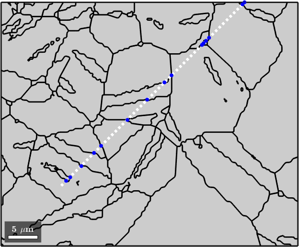

Each blue marker is a reported crossing. Adjacent boundary segments share vertices. A line through a vertex can therefore report the same geometric crossing more than once. Avoid such vertices when placing test lines, or consolidate coincident points before counting them.

Mean lineal intercept

For a traverse of length \(L\) with \(N\) boundary crossings, the mean lineal intercept is \(\bar{\ell} = L/N\). It is a standard measure of apparent grain size. Here the three quantities are printed because they are the result of the example.

nIntersections = nnz(isIntersection)
lineLength = norm(xy2-xy1)
meanIntercept = lineLength / nIntersections

nIntersections =
    18
lineLength =
   43.8406
meanIntercept =
    2.4356

This 43.84 µm traverse crosses 18 boundary segments. Its mean lineal intercept is 2.44 µm. This is apparent grain size on a two-dimensional section, not a mean grain diameter in three dimensions.

From one traverse to a measurement

One line is a thin estimate, and this one runs diagonally across a map full of twin lamellae, every one of which it counts. In practice, add the lengths of many parallel test lines and divide by their total number of crossings. Repeat this measurement in several directions for an elongated microstructure. A line along the elongation crosses fewer boundaries than one drawn across it.

This directional sensitivity is useful, but it means that a single line must not be presented as a direction-independent grain size. A formal measurement also needs a sampling design. Follow the boundary-counting rules of the applicable standard.

A single line still gives a useful reconstruction check. Compare its crossing count with what the grain sizes imply. If they disagree badly, the reconstruction is finding boundaries that are not there, or missing ones that are.

Further reading

Next

A test line samples how often boundaries occur along one chosen direction. Boundary Normal Distribution instead uses many boundary traces to estimate which interface planes are preferred.