In this section we discuss geometric properties of grains that are related to ellipses fitted to the grains. Most importantly these are the centroid c, the long axis a and the short axis b that are computed by the command [c,a,b] = grains.fitEllipse. Based on these quantities the aspectRatio is defined as the quotient a/b between long and short axis.
In order to demonstrate these properties we start by reconstructing the grain structure from a sample EBSD data set.
% load sample EBSD data set
mtexdata forsterite silent

% reconstruct grains and smooth them
[grains, ebsd.grainId] = calcGrains(ebsd('indexed'),'angle',5*degree,'minPixel',10);

grains(grains.isBoundary) = [];

grains = smooth(grains('indexed'),10,'moveTriplePoints');

% plot the grains
plot(grains,'micronbar','off','lineWidth',2)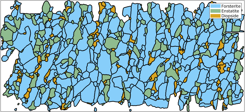
Fit Ellipses
The basic command for fitting ellipses is fitEllipse
[c,a,b] = grains.fitEllipse;

plotEllipse(c,a,b,'lineColor','w','linewidth',2)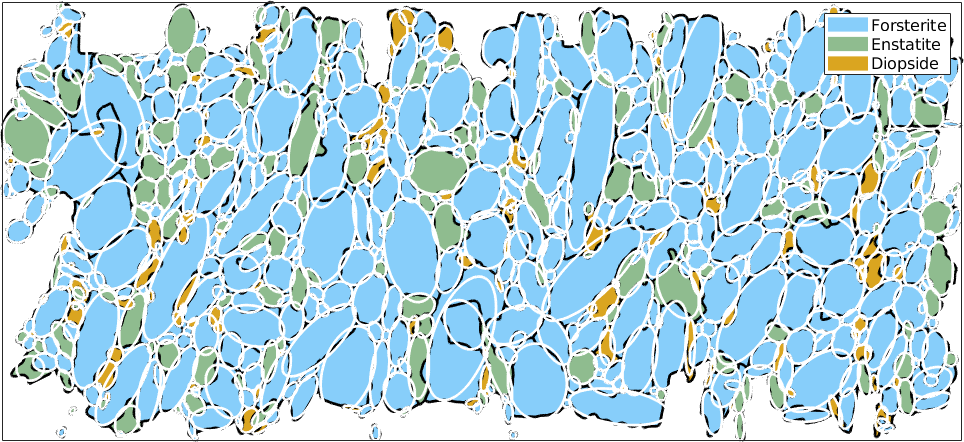
The returned variable c is the centroid of the grains, a and b are of type vector3d and are longest and shortest half axes. Note, that the ellipses are scaled such that the area of the ellipse coincides with the actual grain area. Alternatively, one can also scale the ellipse to fit the boundary length by using the option boundary.
Long and Short Axes
The direction of the long and the short axis of the fitted ellipse can also be obtained by the commands grains.longAxis and grains.shortAxis. These directions are only well defined if the fitted ellipse is not to close to a perfect circle. A measure for how distinct the ellipse is from a perfect circle is the aspect ratio which is defined as the quotient \(a/b\) between the longest and the shortest axis. For a perfect circle the aspect ratio is \(1\) and increases to infinity when the ellipse becomes more and more elongated.
Lets colorize the grains by their aspect ratio and plot on top the long axis directions:
% visualize the aspect ratio
plot(grains,grains.aspectRatio,'linewidth',2,'micronbar','off')
setColorRange([0,4])
mtexColorbar('title','aspect ratio')

% and on top the long axes
hold on
quiver(grains,grains.longAxis,'Color','white')
hold off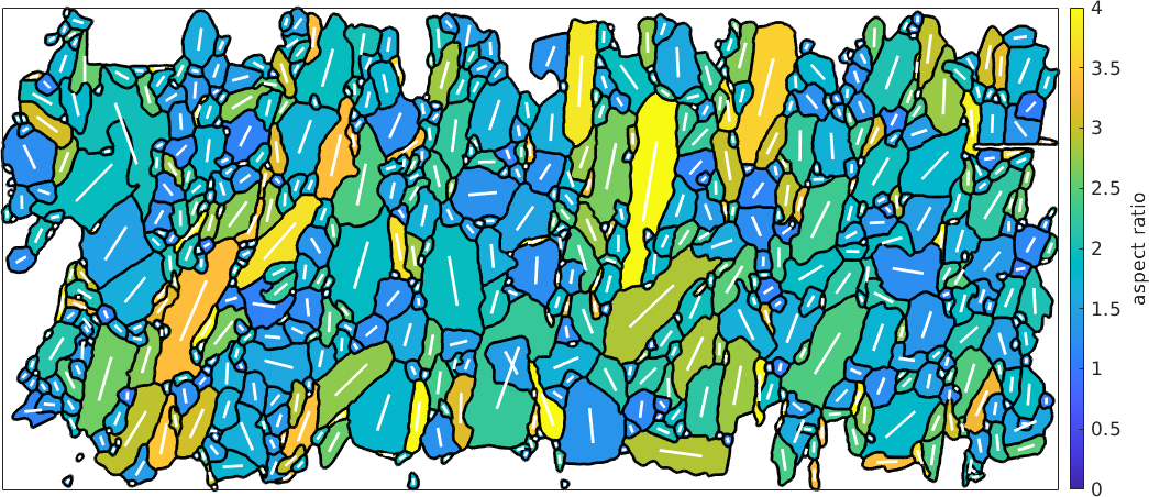
Shape preferred orientation
If we look at grains, we might wonder if there is a characteristic difference in the grain shape fabric between e.g. Forsterite and Enstatite. In contrast to crystal preferred orientations which which describe on the alignment of the atom lattices the shape preferred orientation (SPO) describes the alignment of the grains by shape in the bulk fabric.
Long Axis Distribution
The most direct way to analyze shape preferred orientations are rose diagrams of the distribution of the grain long axes. For those diagrams it is useful to weight the long axis by the grain area such that larger grains have a bigger impact on the distribution and by the aspect ratio as for grains with a small aspect ratio the long axis is not so well defined.
numBin = 50;

subplot(1,2,1)
weights = grains('forsterite').area .* (grains('forsterite').aspectRatio-1);
histogram(grains('forsterite').longAxis,numBin, 'weights', weights)
title('Forsterite')

subplot(1,2,2)
weights = grains('enstatite').area .* (grains('enstatite').aspectRatio - 1);
histogram(grains('enstatite').longAxis,numBin,'weights',weights)
title('Enstatite')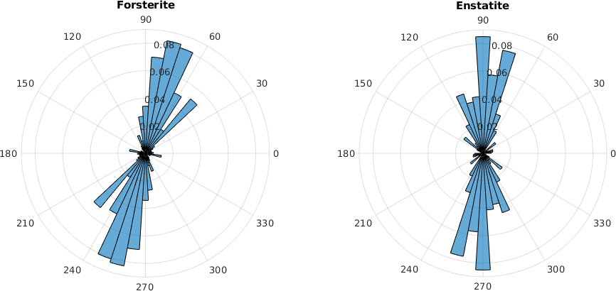
Instead of the histogram we may also fit a circular density distribution to the to the long axes using the command calcDensity.
tdfForsterite = calcDensity(grains('forsterite').longAxis,...
  'weights',norm(grains('forsterite').longAxis));

tdfEnstatite = calcDensity(grains('enstatite').longAxis,...
  'weights',norm(grains('enstatite').longAxis));
Since the input was of type vector3d, the result is a spherical function S2FunHarmonic. We can visualize a section using plotSection|.
close all
plotSection(tdfForsterite, vector3d.Z, 'linewidth', 3)
hold on
plotSection(tdfEnstatite, vector3d.Z, 'linewidth', 3)
hold off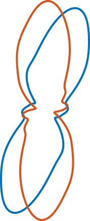
Alternatively, since all vectors are within the plane, only one angle is relevant, one can also compute an S1Fun using vector3d.rho and calcDensity.html|calcDensity| with the option 'periodic'.
tdfForsterite = calcDensity(grains('forsterite').longAxis.rho,...
  'weights',norm(grains('forsterite').longAxis), ...
  'periodic','antipodal','sigma',5*degree);

tdfEnstatite = calcDensity(grains('enstatite').longAxis.rho,...
  'weights',norm(grains('enstatite').longAxis), ...
  'periodic','antipodal','sigma',5*degree);

close all
plot(tdfForsterite, 'linewidth', 2)
hold on
plot(tdfEnstatite, 'linewidth', 2)
hold off
mtexTitle('long axes')
legend('Forsterite','Enstatite','Location','southoutside','numColumns',2)

% we have to set the plotting convention manually
setView(ebsd.how2plot)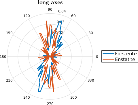
Shortest Caliper Distribution
Alternatively, we may wonder if the common long axis of grains is suitably represented by the direction normal to the shortest caliper of the grains. This can particularly be the case for aligned rectangular particles where the long axes often switch between the diagonals of the particle. The caliper or Feret of grains represents the projection lengths of grains in relation to a projection direction. With the option 'shortestPerp', the function returns the normal to the projection direction with the shortest projection length of a grain. In order to plot the result we could use a histogram, compute a density function or use calcTDF with a list of angles and a list of weights or lengths as input.
cPerpF = caliper(grains('fo'),'shortestPerp');
cPerpE = caliper(grains('en'),'shortestPerp');

S1F_fo = calcDensity(cPerpF.rho, 'weights',cPerpF.norm, ...
  'periodic','antipodal','sigma',5*degree);
S1F_en = calcDensity(cPerpE.rho, 'weights',cPerpE.norm,...
  'periodic','antipodal','sigma',5*degree);

plot(S1F_fo,'linewidth',2);
hold on
plot(S1F_en,'linewidth',2);
hold off
mtexTitle('perpendicular to short axes')
legend('Forsterite','Enstatite','Location','southoutside','numColumns',2)
setView(ebsd.how2plot)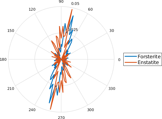
If we consider the function a little to rough, we can smooth the function using a kernel.
psi = S1DeLaValleePoussinKernel('halfwidth',10*degree)

S1_fo_smooth = conv(S1F_fo,psi)
S1_en_smooth = conv(S1F_en,psi)

plot(S1_fo_smooth,'linewidth',2);
hold on
plot(S1_en_smooth,'linewidth',2);
hold off
mtexTitle('perpendicular to short axes')
legend('Forsterite','Enstatite','Location','southoutside','numColumns',2)
setView(ebsd.how2plot)
psi = S1DeLaValleePoussinKernel
bandwidth: 14
halfwidth: 9.9°
S1_fo_smooth = S1FunHarmonic
bandwidth: 14
antipodal: true
isReal: true
S1_en_smooth = S1FunHarmonic
bandwidth: 14
antipodal: true
isReal: true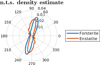
SPO defined by grain boundary segments
Best fit ellipses are always symmetric and the projection function of an entire grain always only consider the convex hull. Grain shape fabrics can also be characterized by a rose diagram of the directions of grain boundary segments which can consider the entire shape of the grain defined by the grain boundary segments but also works for non fully enclosed shapes i.e. just a special selection of grains. Here, we can weight each direction > of a grain boundary by its <grainBoundary.segLength.html segment length|.
Let's compare different types of boundaries
gbfun_fofo = calcDensity(grains.boundary('fo','fo').direction.rho, ...
    'weights',grains.boundary('fo','fo').segLength,'periodic','antipodal');
gbfun_foen = calcDensity(grains.boundary('fo','en').direction.rho, ...
    'weights',grains.boundary('fo','en').segLength,'periodic','antipodal');
gbfun_enen = calcDensity(grains.boundary('en','en').direction.rho, ...
    'weights',grains.boundary('en','en').segLength,'periodic','antipodal');

plot(gbfun_fofo,'displayName','Forsterite-Forsterite','linewidth',2);
hold on
plot(gbfun_foen,'displayName','Forsterite-Enstatite','linewidth',2);
hold on
plot(gbfun_enen,'displayName','Enstatite-Enstatite','linewidth',2);
hold off

legend('Location','eastoutside','numColumns',1)

setView(ebsd.how2plot)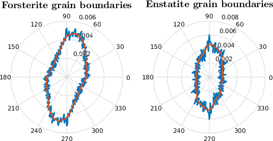
Characteristic Shape
Note that this distribution is very prone to inherit artifacts based on the fact that most EBSD maps are sampled on a regular grid. We tried to overcome this problem by heavily smoothing the grain boundary. However, if you recognize little peaks at 0 and 90 degree, they are most likely related to this sampling artifact.
If we just add up all the individual boundary elements of the rose diagram in order of increasing angles, we derive the characteristic shape. It can be regarded as to represent the average grain shape. The < grainBoundary.characteristicShape.html characteristicShape>does not require entire grains as input but works with a list of grain boundaries. Many operations such as aspectRatio or longAxis also work on the characteristic shape.
cshapeF = characteristicShape(grains('F').boundary);
cshapeE = characteristicShape(grains('E').boundary);

close all
plot(cshapeF, 'linewidth',2);
hold on
plot(cshapeE, 'linewidth',2);
hold off
legend('Forsterite','Enstatite','Location','eastoutside')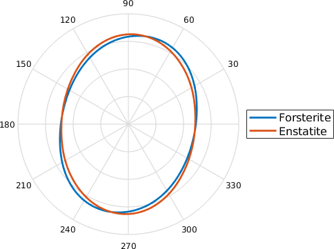
We may wonder if these results are significantly different or not TODO: get deviation from an ellipse etc