3D Orientation Visualizations

What a Three-Dimensional Point Retains

A pole figure shows one crystal direction and discards the rest of the orientation. A three-dimensional orientation plot instead assigns one point to all three rotational degrees of freedom. Nothing is lost, but the plot has to be rotated to reveal occluded points.

This page assumes the crystal-to-specimen map from Theory, the symmetry-equivalent representatives from Symmetry, and the rotation coordinates from Rotation Representations.

A plotting convention states how a reference frame is laid out on screen. The convention below draws Y upward and X to the right. It changes the screen layout, not the orientations or their reference frames.

plottingConvention.default('y↑→x');

cs = crystalSymmetry('cubic');

ori = orientation.rand(100,cs);

Euler Angle Space

plot with 'Bunge' places each orientation at its three Bunge Euler angles \((\varphi_1,\Phi,\varphi_2)\).

plot(ori,'Bunge')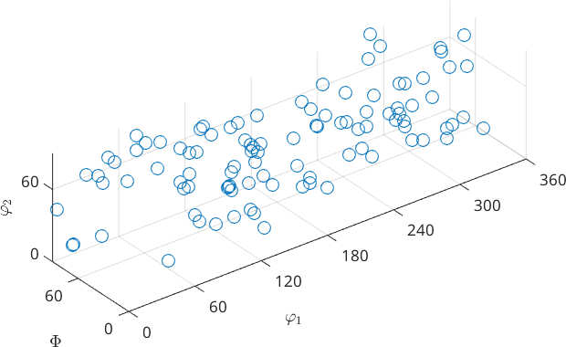

MTEX first selects one symmetry-equivalent representative in the fundamental region. For cubic crystal symmetry and identity specimen symmetry, \(\Phi\) and \(\varphi_2\) stop at \(90^\circ\), while \(\varphi_1\) still runs to \(360^\circ\). Every orientation outside this box has an equivalent representative inside, so the reduction hides no orientations. See Fundamental Regions.

The flag 'ignoreFundamentalRegion' instead draws the stored representatives at their unreduced Euler angles.

plot(ori,'Bunge','ignoreFundamentalRegion')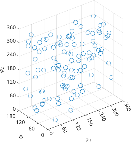

The same cloud now fills the full \(360^\circ\) by \(180^\circ\) by \(360^\circ\) Euler box. The points outside the smaller box are not new or invalid orientations; symmetry would move each one back inside.

Notice how the points thin out towards \(\Phi=0\). A uniform orientation distribution is not uniform in these rectangular coordinates because its volume element contains \(\sin\Phi\). A cluster near \(\Phi=0\) is therefore not as concentrated as it looks.

The rectangular geometry is only a coordinate chart. Do not use the Euclidean distance between two plotted points as their angular separation; use angle on the orientations themselves.

Axis--Angle Space

A second common view uses the scaled-axis vector

\[ \mathbf{r}=\omega\mathbf{n}, \]

where the direction \(\mathbf{n}\) is the rotation axis and the distance \(\omega\) from the origin is the rotation angle of the selected representative.

plot(ori,'axisAngle','markerEdgeColor',[0 0 0.8],'markerSize',8)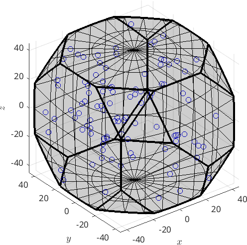

All points lie inside the automatically drawn fundamental region. Unlike the Euler box, its boundary is a polyhedron-like surface whose radial distance depends on the rotation axis.

Drawing the unreduced representatives together with the region makes the effect of symmetry reduction explicit.

plot(ori,'axisAngle','ignoreFundamentalRegion',...
  'markerEdgeColor',[0 0 0.8],'markerSize',8)

% visualize the fundamental region
hold on
oR = fundamentalRegion(ori.CS,ori.SS);
plot(oR,'color',[1 0.5 0.5])
hold off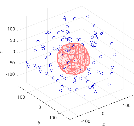

The blue points outside the red solid are the representatives that the previous plot moved inside. They remain physically equivalent to points within the region.

Axis--angle space is the more faithful of these two views: radial distance is a rotation angle, and it distorts volume far less than Euler space. It still does not preserve volume or make every Euclidean point distance an orientation angle. Its direct geometric reading is why it is the default three-dimensional view for misorientations.

MTEX can also draw 'Rodrigues', 'homochoric', and 'cubochoric' coordinates. Rodrigues coordinates make several symmetry boundaries planar, while homochoric and cubochoric coordinates preserve orientation volume. Rotation Representations compares these choices and their appropriate uses.

References

Next

Dense orientation data are usually read as two-dimensional cuts through these spaces; continue with Section Plots. The shape and symmetry of the region are developed in Fundamental Regions. The next chapter applies the axis--angle view to relative orientations in Misorientations.

References

- H.-J. Bunge, Texture Analysis in Materials Science: Mathematical Methods, Butterworths, English ed., 1982, develops Bunge Euler space and orientation distributions.
- A. Morawiec, Orientations and Rotations: Computations in Crystallographic Textures, Springer, 2004, treats rotation-space geometry, parametrisations, and symmetry domains.
- D. Rowenhorst et al., Consistent representations of and conversions between 3D rotations, Modelling and Simulation in Materials Science and Engineering 23 (2015), 083501, compares the conventions and tradeoffs of common rotation representations.