Approximation of Orientation Dependent Functions

Assume we have given some evaluation routine \(f\) that maps orientations to numbers. This could be an rotational function of class SO3Fun, a @function_handle, a more complex Matlab function or a physical experiment.

On this page we will explain how to compute the corresponding SO3FunHarmonic and SO3FunRBF that approximates \(f\) reasonable well.

This approximation process is similarly to Approximating Orientation Dependent Functions from Discrete Data. where the given data are a set of orientations with function values.

Lets load an orientation dependent function as SO3Fun.

mtexdata dubna
odf = calcODF(pf,'resolution',5*degree,'zero_Range')
plot(odf,'sigma')

In the following we will differentiate whether we approximate \(f\) by a SO3FunHarmonic or by a SO3FunRBF.

Harmonic Approximation

The basic strategy is to approximate the data by a SO3FunHarmonic (Harmonic series), i.e. a series of Wigner-D functions, see SO3FunHarmonicSeries Basics of rotational harmonics.

For that, we compute the so-called Fourier coefficients \({\bf \hat f} = (\hat f^{0,0}_0,\dots,\hat f^{N,N}_N)^T\) of

\[ f({\bf R}) = \sum_{n=0}^N\sum_{k,l=-n}^n \hat{f}^{k,l}_n \, D_n^{k,l}({\bf R}). \]

The Fourier coefficients are defined by

\[ \hat f^{k,l}_n = \int_{SO(3)} f({\bf R}) \cdot \overline{D_n^{k,l}({\bf R})} \mathrm{d}\my({\bf R}) \]

and we compute this integral by numerical integration, which is also called quadrature, i.e.

\[ \hat f^{k,l}_n \approx \sum_{m=1}^M \omega_m \, f({\bf R}_m) \, \overline{D_n^{k,l}({\bf R}_m)} \]

with suitable quadrature weights \(\omega_m\) and quadrature nodes \(\bf{R}_m\), \(m=1,\dots,M\).

In MTEX there are two quadrature schemes predefined:

Both of them are defined with respect to some bandwidth \(N\) and they are exact for all band-limited functions of this specific bandwidth. That means, if we perform quadrature on any SO3FunHarmonic of bandwidth N with one of this schemes, then we will get exactly this function back.

In MTEX we use the command SO3FunHarmonic to expand any SO3Fun or @function_handle into an SO3FunHarmonic.

SO3F = SO3FunHarmonic(odf)
plot(SO3F,'sigma')

Internally MTEX calls SO3FunHarmonic.approximate. We can specify the bandwidth of the approximated SO3FunHarmonic with the option 'bandwidth' and we can tell MTEX to use the other quadrature scheme.

SO3F = SO3FunHarmonic(odf,'bandwidth',10,'GaussLegendre')
plot(SO3F,'sigma')

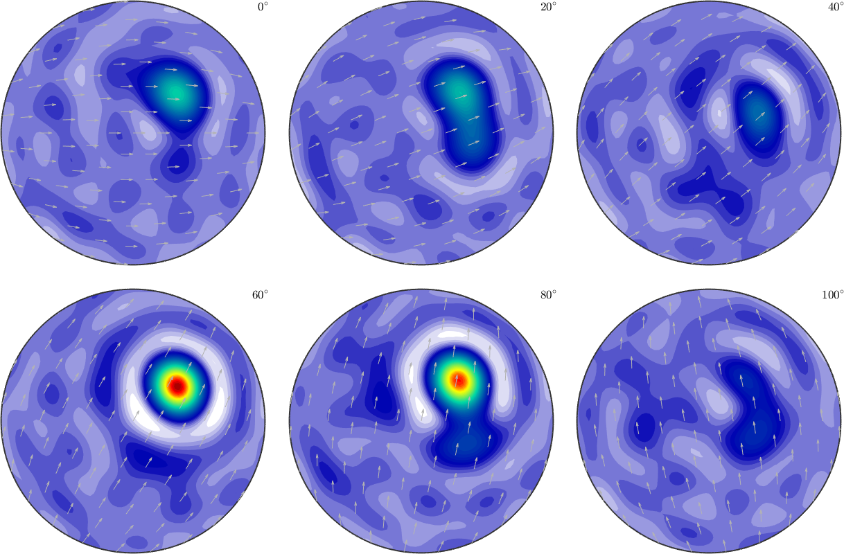
If we do not have an SO3Fun or @function_handle, but we try to approximate a function from some physical experiment or more complex Matlab function (where we can put in specific orientations and get out numbers), then we proceed as follows.

One idea could be to perform the experiment for random orientations and interpolate this discrete data in a second step.

But, if we can choose the orientations by our own, we should better choose an optimal/minimal orientation grid, perform the experiment on this grid and compute the Fourier coefficients of the harmonic expansion by quadrature.

This is exactly what happens internally when we call the SO3FunHarmonic-command. In fact this is a special case of approximation of discrete data for a very specific grid.

% Specify the bandwidth and symmetries of the desired harmonic odf
bw = 50;
cs = crystalSymmetry('321');
ss = specimenSymmetry;

% Compute the quadrature grid and weights
CC_grid = quadratureSO3Grid(bw,'ClenshawCurtis',cs,ss);

% Because of symmetries there are symmetric equivalent nodes in the
% quadrature grid. Hence we perform our experiment on a smaller unique
% grid.
ori = CC_grid(:)
v = EXPERIMENT(ori);

% At the end we do quadrature
E1 = SO3FunHarmonic.quadrature(CC_grid,v)
% E1 = SO3FunHarmonic.interpolate(CC_grid,v) % does the same

Furthermore, if the experimental step is very expansive it might be a good idea to use the smaller Gauss-Legendre quadrature grid. The Gauss-Legendre quadrature lattice has half as many points as the default Clenshaw-Curtis quadrature lattice. But the quadrature method is slightly more time consuming.

% Compute the Gauss-Legendre quadrature grid and weights
GL_grid = quadratureSO3Grid(bw,'GaussLegendre',cs,ss);

% Perform the experiment on that quadrature grid
ori = GL_grid(:)
v = EXPERIMENT(ori);

% Do quadrature
E2 = SO3FunHarmonic.quadrature(GL_grid,v)

Both of this quadrature schemes yield exactly the same SO3FunHarmonic.

calcError(E1,E2)

RBF-Kernel Approximation

The basic strategy is to approximate the given function \(f\) by a SO3FunRBF, see Radial Basis Functions on SO(3).

Hence we determine rotations \(R_1,\dots,R_N\) and seek the corresponding coefficients \(\vec c=(c_1,\dots,c_N)\) such that

\[ g(x) = \sum_{n=1}^N c_n \, \Psi(\cos\frac{\omega(x,R_n)}{2}) \]

approximates \(f\) reasonable well, i.e. \(f\approx g\). In this formula, \(\Psi\) describes a SO(3)-Kernel Function. Hence, \(f\) is a superposition of one rotational kernel function centered on the orientations \(R_1,\dots,R_N\) and weighted by the coefficients \(c_1,\dots,c_N\).

A basic strategy is to apply least squares approximation, where we compute the coefficients \(c_n\) by minimizing the functional

\[ \sum_{m=1}^M|f(x_m)-g(x_m)|^2 \]

for some specific orientations \(x_1,\dots,x_M\).

This least squares problem can also be written in matrix vector notation \( \argmin_{c} \| K \cdot c - v \|, \) where \(x=(c_1,\dots,c_N)^T\), \(v=(v_1,\dots,v_M)^T\) and \(K\) is the kernel matrix \([\Psi(\cos\frac{\omega(x_m,R_n)}{2})]_{m,n}\).

This least squares problem can be solved by the lsqr method from MATLAB, which efficiently seeks for roots of the derivative of the given functional (also known as normal equation).

Alternatively there is also a modified least square method mlsq, which search for a solution \(c_1,\dots,c_N\) that satisfies \(c>0\) and \(\sum_{n=1}^N c_n = 1\). This method can be used if the underlying function is a density, i.e. it is nonnegative and has mean 1, which can be applied if we try to approximate a density function.

In MTEX we use the command SO3FunRBF to represent any SO3Fun or @function_handle by an SO3FunRBF.

SO3F3 = SO3FunRBF(odf,'density')
% SO3F3 = SO3FunRBF.approximate(odf,'density')
plot(SO3F3,'sigma')

Here MTEX internally calls the SO3FunRBF.approximate method.

The flag 'density' tells MTEX to use the mlsq solver, which ensures that the resulting function is nonnegative and normalized to mean \(1\).

minValue = min(SO3F3)

meanValue = mean(SO3F3)

We can specify the kernel of the approximated SO3FunRBF with the option 'kernel' or 'halfwidth' and we can use the options 'SO3Grid' and 'resolution' to choose some specific set of rotations as centers \(R_1,\dots,R_N\) of the approximation \(g\).

SO3F4 = SO3FunRBF(odf,'halfwidth',5*degree,'resolution',10*degree)
plot(SO3F4,'sigma')

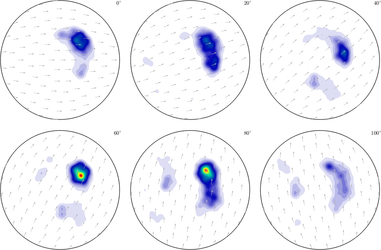
S3G = orientation.rand(1000,odf.CS);
psi = SO3AbelPoissonKernel('halfwidth',5*degree);
SO3F5 = SO3FunRBF(odf,'kernel',psi,'SO3Grid',S3G)
plot(SO3F5,'sigma')

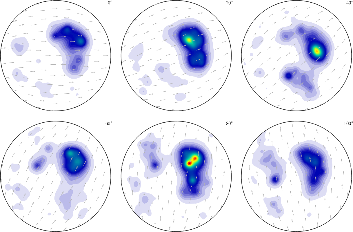
SO3F6 = SO3FunRBF(odf,'halfwidth',5*degree,'approxresolution',5*degree)
plot(SO3F6,'sigma')

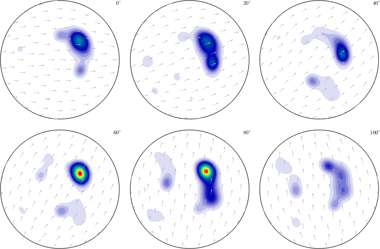
The errors are

calcError(odf,SO3F3)
calcError(odf,SO3F4)
calcError(odf,SO3F5)
calcError(odf,SO3F6)

If we do not have an SO3Fun or @function_handle, but we try to approximate a function from some physical experiment or more complex Matlab function (where we can put in specific orientations and get out numbers), then we should perform the experiment for all orientations of an @equispacedSO3Grid and approximate this discrete data in a second step.

RBF-Kernel Approximation by minimizing the harmonic Error

The basic idea is the same as in the previous section. We determine rotations \(R_1,\dots,R_M\) and seek the corresponding coefficients \(\vec c=(c_1,\dots,c_N)\) of

\[ g(x) = \sum_{m=1}^M c_m \, \Psi(\cos\frac{\omega(x,R_m)}{2}), \]

such that \(g\) approximates \(f\) in a certain sense. But in what sense exactly?

In the previous section, we minimized the pointwise error (in spatial domain) between \(f\) and \(g\) on some grid, i.e. we minimized \( \ds \sum_{m=1}^M|f(x_m)-g(x_m)|^2 \) in \(M\) points.

Now we will minimize the error in frequency domain. Hence, the Fourier coefficients of \(f\) are supposed to be nearly the same as the Fourier coefficients of \(g\).

So, we will try to determine the coefficients \(c_1,\dots,c_M\) such that

\[ \sum_n=0^N \sum_{k,l=-n}^n (\hat f_n^{k,l} - \hat g_n^{k,l})^2 \]

is minimized.

In MTEX we call this by adding the option 'harmonic' to the SO3FunRBF-command.

SO3F7 = SO3FunRBF(odf,'harmonic')
plot(SO3F7,'sigma')

LSQR-Parameters

The lsqr solver and the mlsq solver, which are used to minimize the least squares problem from above has some predefined termination conditions. We can specify the method tolerance with the option 'tol' (default 1e-3) and the maximum number of iterations by the option 'maxit' (default 30/100).

Thus we are able to control the precision of the result and computational time of the least squares methods in the approximation process.

function v = EXPERIMENT(ori)
  v = SO3Fun.dubna.eval(ori);
end