Plotting Rotations

A single rotation is best drawn by what it does, as in Defining Rotations. A set of rotations needs a different picture. Each rotation becomes one point in a three-dimensional coordinate domain, with the domain determined by the parametrisation.

This page assumes the axis--angle and Bunge Euler descriptions introduced in Defining Rotations. The geometric trade-offs between coordinate systems are developed in Rotation Representations.

The plotting convention controls how the reference frame is laid out on screen. This page uses y north and x east.

plottingConvention.default('y↑→x');

rot = rotation.rand(500);

Euler Angle Space

scatter places each rotation at its three Bunge Euler angles. This is the default for rotations without crystal symmetry. The complete box spans \(0\leq\varphi_1,\varphi_2\leq2\pi\) and \(0\leq\Phi\leq\pi\).

scatter(rot,'Bunge')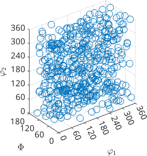

The sample is uniform in rotation space, but its points are not uniform in this box. Notice how the cloud thins near both \(\Phi=0\) and \(\Phi=\pi\). Equal-sized boxes at different values of \(\Phi\) represent different volumes of rotation space. Point density in an Euler plot is therefore not itself a texture density.

Axis--Angle Space

Axis--angle coordinates place a rotation at \(\omega\vec n\). The direction \(\vec n\) is its rotation axis and the distance from the origin is its principal rotation angle \(\omega\).

scatter(rot,'axisAngle')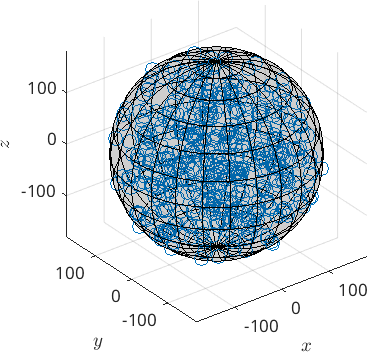

The identity is at the centre and half turns lie on the outer sphere. Most of the points lie beyond half the radius, because a uniform sample contains more large-angle rotations than small-angle rotations. Opposite points on the outer sphere describe the same \(180^\circ\) rotation.

Rodrigues--Frank Space

Rodrigues--Frank coordinates keep the direction \(\vec n\) but change the distance from the origin to \(\tan(\omega/2)\).

scatter(rot,'Rodrigues','noBoundary')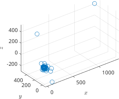

Rotations near \(180^\circ\) now lie far from the centre, so they stretch the plot and compress the appearance of the remaining cloud. Half turns themselves are at infinity. This domain makes fixed-axis rotations and symmetry boundaries simple, but it does not preserve volume.

In all three plots, coordinate distance should not be read as the angular distance between arbitrary rotations. Use angle for that comparison. Homochoric and cubochoric coordinates preserve volume instead; see Rotation Representations.

Highlighting a Subset

The usual marker options can distinguish a selected subset. Here the red points are rotations less than \(60^\circ\) from the identity.

threshold = 60*degree;
small = rot(rot.angle < threshold);

scatter(rot,'axisAngle','MarkerFaceColor',[.7 .7 .7],'MarkerSize',4)
hold on
scatter(small,'axisAngle','MarkerFaceColor','r')
hold off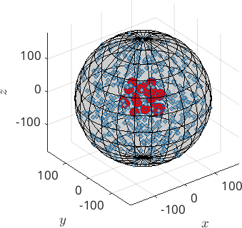

The red points form a ball around the identity. Count them and report the fraction rather than estimating either value from the figure.

numSmall = length(small)
empiricalPercent = 100 * numSmall / length(rot)

numSmall =
    24
empiricalPercent =
    4.8000

This reproducible draw contains 20 of 500 rotations, or 4%. Sampling variation explains why it does not equal the population value below.

Why Uniform Rotations Look Nonuniform

Uniform means uniform with respect to the invariant, or Haar, measure on the rotation group. In Bunge Euler angles its normalized volume element is

\[\mathrm{d}g = \frac{1}{8\pi^2}\sin\Phi\, \mathrm{d}\varphi_1\,\mathrm{d}\Phi\,\mathrm{d}\varphi_2.\]

The factor \(\sin\Phi\) explains the emptying of the Euler box near its two \(\Phi\) faces. In axis--angle coordinates the fraction of all rotations with angle at most \(\omega\) is

\[P(\Omega\leq\omega)=\frac{\omega-\sin\omega}{\pi}.\]

At \(60^\circ\), this exact fraction is

exactPercent = 100 * (threshold - sin(threshold)) / pi

exactPercent =
    5.7669

The result is 5.7669%. Even this broad \(60^\circ\) ball occupies only a small part of rotation space. A scatter plot shows sampled coordinates; estimating a continuous texture density requires calcDensity.

Further Reading

Next

An orientation combines a rotation with crystal and specimen symmetry. Its scatter plot is restricted to a fundamental region by default. Dense orientation sets are usually clearer as sections through that region; see Section Plots.