This page describes how to use MTEX to estimate an ODF from pole figure data. Starting point of any ODF reconstruction is a PoleFigure object which can be created e.g. by
mtexdata dubnapf = PoleFigure (y↑→x)
crystal symmetry : Quartz (321, X||a*, Y||b, Z||c*)
h = (022̅1), r = 72 x 19 points
h = (101̅0), r = 72 x 19 points
h = (101̅1)(011̅1), r = 72 x 19 points
h = (101̅2), r = 72 x 19 points
h = (112̅0), r = 72 x 19 points
h = (112̅1), r = 72 x 19 points
h = (112̅2), r = 72 x 19 pointsSee Import for more information how to import pole figure data and to create a pole figure object.
% plot pole figures
plot(pf)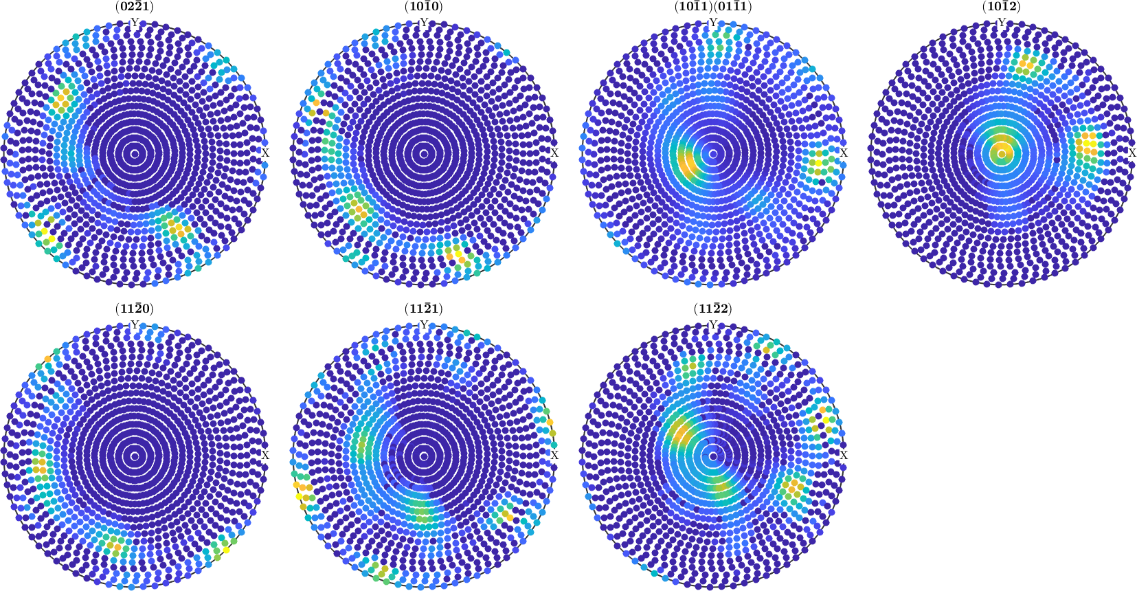
ODF Estimation
ODF estimation from a pole figure object is done by the function calcODF. The most simplest syntax is
odf = calcODF(pf)odf = SO3FunRBF (Quartz → y↑→x)
multimodal components
kernel: de la Vallee Poussin, halfwidth 5°
center: 19848 orientations, resolution: 5°
weight: 1There are a lot of options to the function calcODF. You can specify the discretization, the functional to minimize, the number of iteration or regularization to be applied. Furthermore, you can specify ghost correction or the zero range method to be applied. These options are discussed below.
You may want to verify that the pole figures are reproduced. Here is a plot of the computed pole figures.
plotPDF(odf,pf.allH,'antipodal','silent','superposition',pf.c)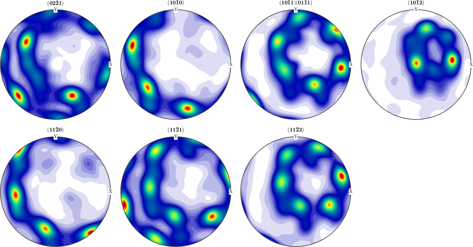
Error analysis
For a more quantitative description of the reconstruction quality, one can use the function calcError to compute the fit between the reconstructed ODF and the measured pole figure intensities. The following measured are available:
- RP - error
- L1 - error
- L2 - error
calcError(pf,odf,'RP',1)ans =
1.0451 1.0343 0.3712 0.4963 0.6885 0.7009 0.5839In order to recognize bad pole figure intensities, it is often useful to plot difference pole figures between the normalized measured intensities and the recalculated ODF. This can be done by the command plotDiff.
plotDiff(pf,odf)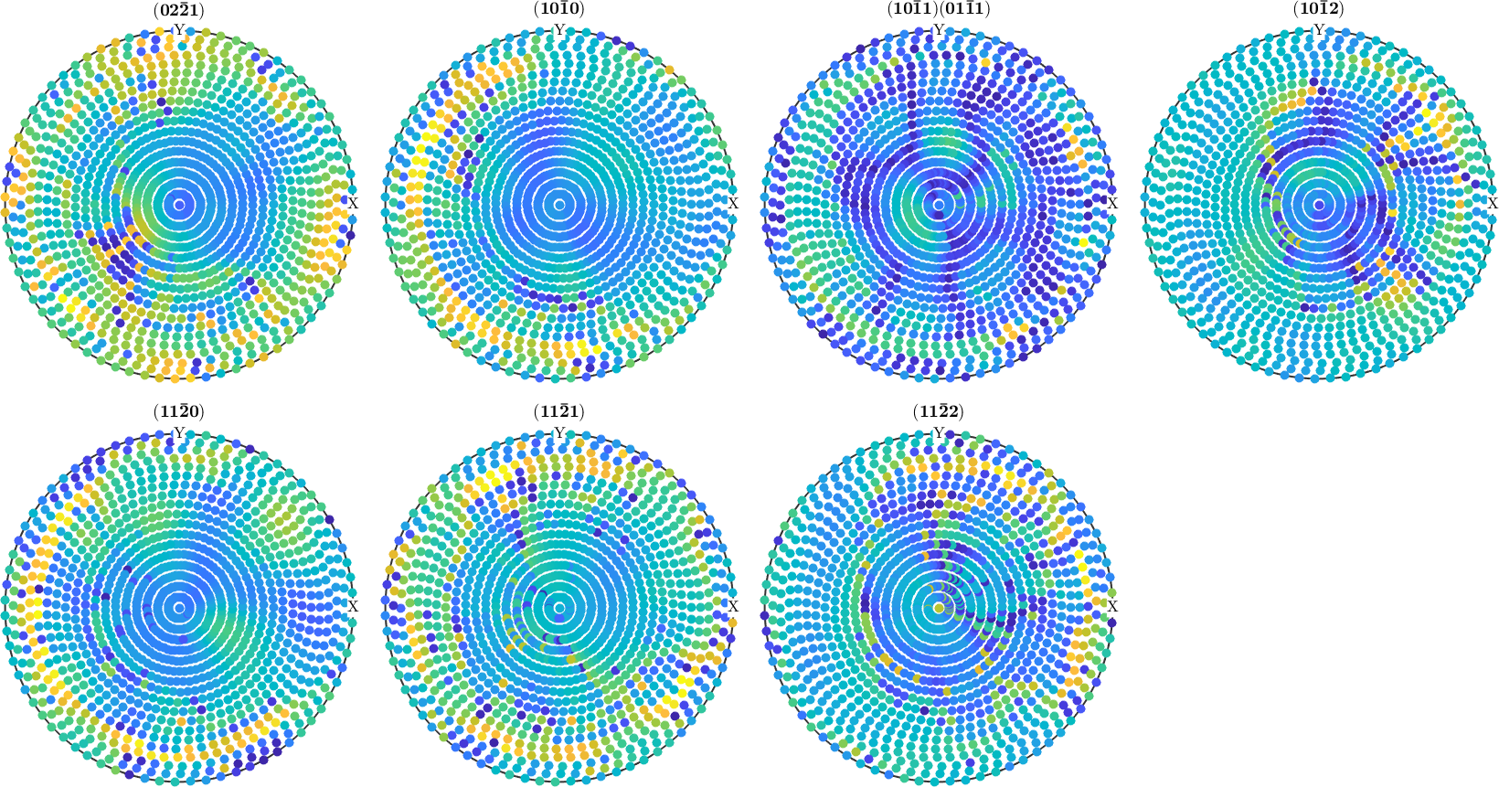
Assuming you have driven two ODFs from different pole figure measurements or by ODF modeling. Then one can ask for the difference between both. This difference is computed by the command calcError.
% define a unimodal ODF with the same preferred orientation
[~,ori_pref] = max(odf);
odf_model = unimodalODF(ori_pref,'halfwidth',15*degree)

% plot the pole figures
plotPDF(odf_model,pf.allH,'antipodal','superposition',pf.c)

% compute the difference
calcError(odf_model,odf)
odf_model = SO3FunRBF (Quartz → y↑→x)
unimodal component
kernel: de la Vallee Poussin, halfwidth 15°
center: 1 orientations
Bunge Euler angles in degree
phi1 Phi phi2 weight
133.047 34.5158 207.16 1
ans =
0.6207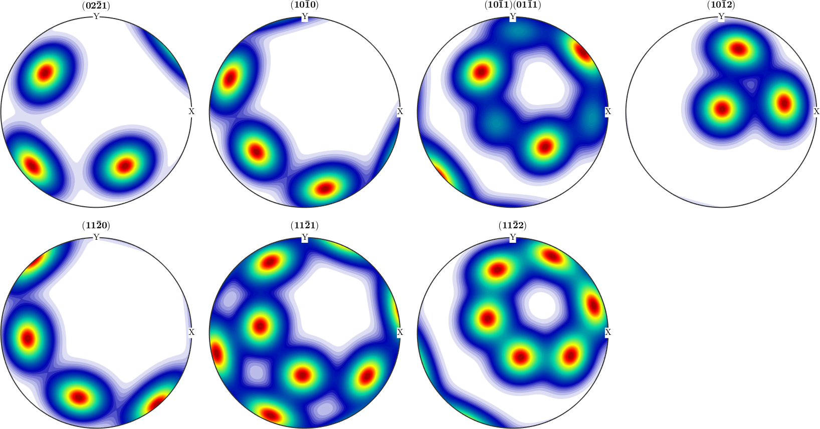
Discretization
In MTEX the ODF is approximated by a superposition of up to 10,000,000 unimodal components. By exact number and position of these components, as well as its shape can be specified by the user. By default, the positions are chosen equispaced in the orientation space with 1.5 times the resolution of the pole figures and the components are de la Vallee Poussin shaped with the same halfwidth as the resolution of the positions.
Next an example how to change the default resolution:
odf = calcODF(pf,'resolution',15*degree)
plotPDF(odf,pf.allH,'antipodal','silent','superposition',pf.c)
odf = SO3FunRBF (Quartz → y↑→x)
multimodal components
kernel: de la Vallee Poussin, halfwidth 15°
center: 736 orientations, resolution: 15°
weight: 1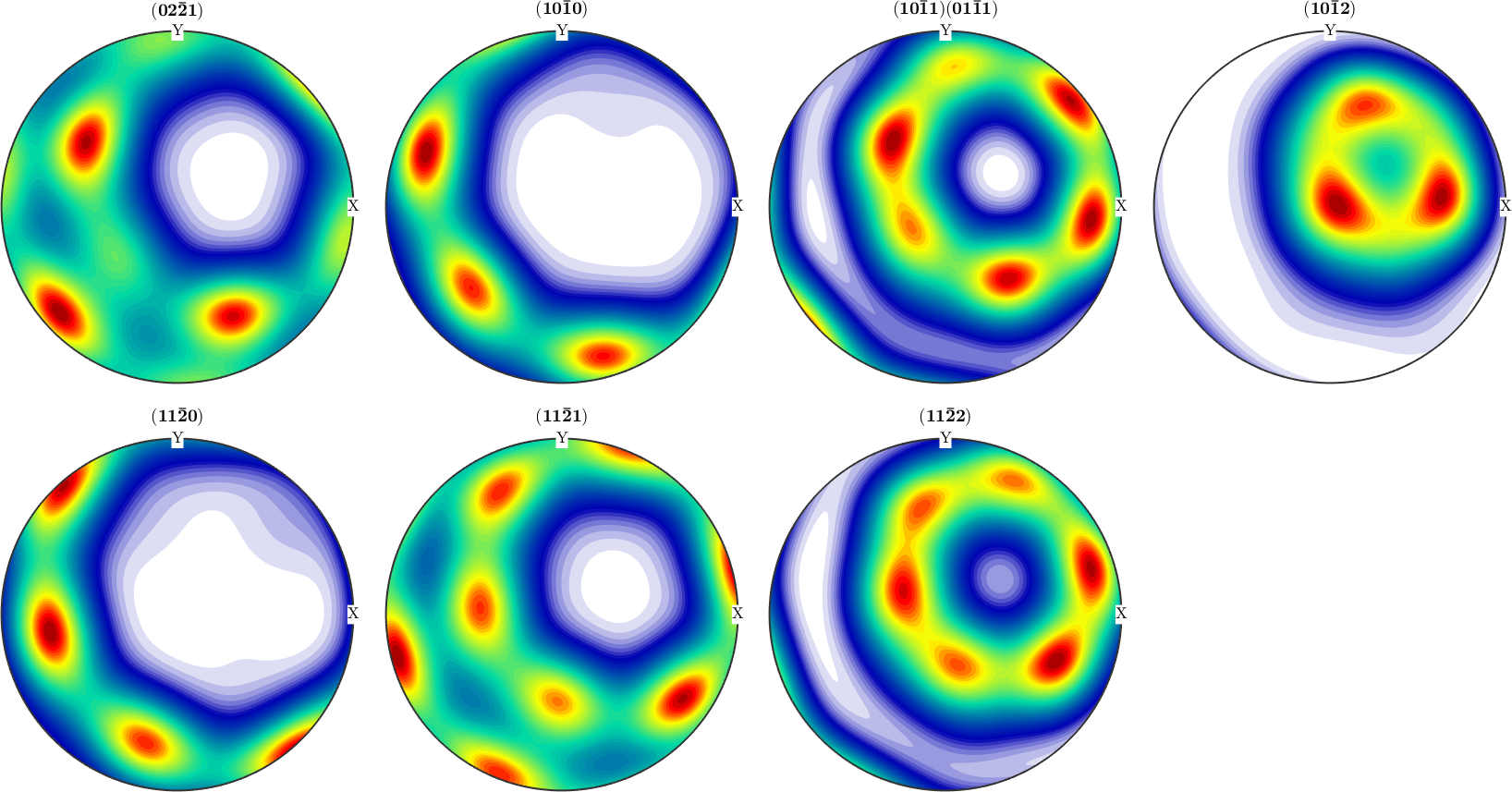
Beside the resolution you can use the following options to change the default discretization:
-
'kernel'to specify a specific kernel function -
'halfwidth'to take the default kernel with a specific halfwidth
Zero Range Method
If the flag 'zero_range' is set the ODF is forced to be zero at all orientation where there is a corresponding zero in the pole figure. This technique is especially useful for sharp ODF with large areas in the pole figure being zero. In this case, the calculation time is greatly improved and much higher resolution of the ODF can be achieved.
In the following example, the zero range method is applied with a threshold 100. For more options to control the zero range method see the documentation of zero_range or zeroRangeMethod.plot.
odf = calcODF(pf,'zero_range')
plotPDF(odf,pf.allH,'antipodal','silent','superposition',pf.c)
odf = SO3FunRBF (Quartz → y↑→x)
multimodal components
kernel: de la Vallee Poussin, halfwidth 5°
center: 19848 orientations, resolution: 5°
weight: 1
Ghost Corrections
Ghost correction is a technique first introduced by Matthies that increases the uniform portion of the estimated ODF to reduce the so called ghost error. It applies especially useful in the case of week ODFs. The classical example is the Santa Fe model ODF. An analysis of the approximation error under ghost correction can be found here
Theory
ODF estimation in MTEX is based upon the modified least squares estimator. The functional that is minimized is
\[f_{est} = argmin \sum_{i=1}^N \sum_{j=1}^{N_i}\frac{|\alpha_i R f(h_i,r_{ij}) - I_{ij})|^2}{I_{ij} }\]
A precise description of the estimator and the algorithm can be found in the paper Pole Figure Inversion - The MTEX Algorithm.