Tensor Visualization

A tensor stores a directional material property, but its component table rarely gives an immediate picture of the anisotropy. This page shows how MTEX turns a tensor into a scalar function on the sphere and how to read the resulting plots.

This page assumes the tensor ranks and physical classes introduced in Defining Tensorial Properties. Read Tensor Arithmetic first if tensor contraction or eigenvectors are new.

A reference frame is the coordinate system in which the tensor is expressed. The plotting convention lays that frame out on screen; it does not rotate the tensor. See Crystal Reference System for the relation between crystal axes and Cartesian axes.

plottingConvention.default('y↑→x');
setMTEXpref('defaultColorMap',blue2redColorMap);

Plotting the directional magnitude

The simplest tensor plot assigns one scalar to every unit direction. MTEX calls this scalar the directional magnitude. plot draws it as a spherical function.

The example is the stiffness tensor of olivine measured by Abramson et al. (1997). Its printed summary records the rank, unit, crystal frame, and coefficients that the plot below represents.

cs = crystalSymmetry('mmm',[4.7646 10.2296 5.9942],...
  'mineral','Olivine');
C = stiffnessTensor.load(...
  fullfile(mtexDataPath,'tensor','Olivine1997PC.GPa'),cs)

C = stiffnessTensor (Olivine)
  unit: GPa              
  rank: 4 (3 × 3 × 3 × 3)
 
  tensor in Voigt matrix representation:
 320.5  68.2  71.6     0     0     0
  68.2 196.5  76.8     0     0     0
  71.6  76.8 233.5     0     0     0
     0     0     0    64     0     0
     0     0     0     0    77     0
     0     0     0     0     0  78.7

plot(C,'complete','upper');
mtexColorbar('title','directional magnitude in GPa');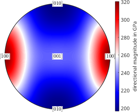

The red maximum lies along \([100]\), while the blue minimum lies along \([010]\). The repeated pattern reflects the orthorhombic crystal symmetry. The options 'complete' and 'upper' show the complete upper hemisphere instead of only the symmetry-reduced sector.

This plot shows the self-contraction of C. It is not Young's modulus or a complete picture of the stiffness tensor. Use YoungsModulus when that physical property is the question.

Inspecting the spherical function

directionalMagnitude returns the spherical function used by plot. The object display identifies its representation, symmetry, bandwidth, and antipodal character.

sF = C.directionalMagnitude

sF = S2FunHarmonicSym (Olivine)
  bandwidth: 4
  antipodal: true

Spherical-function operations can now be applied directly. For example, max finds the largest value and its direction.

[maxValue,maxDirection] = max(sF);
maxDirection = round(maxDirection);
maxValue
maxDirection

maxValue =
  320.5000
 
maxDirection = Miller (Olivine)
 antipodal: true
  h k l
  1 0 0

The output gives a maximum of 320.5 GPa along \([100]\), which is the red direction in the first figure. The spherical plotting options and every spherical projection also apply to sF.

Rank-two tensors and principal axes

For a symmetric rank-two tensor, the directional magnitude is a quadratic form. Its extrema lie along the principal axes, which are the eigenvectors returned by eig.

T = tensor(diag([3 1 -1]),'rank',2);
[e,lambda] = eig(T)

plot(T,'complete','upper');
mtexColorbar('title','directional magnitude');

e = vector3d (y↑→x)
 size: 3 × 1
 antipodal: true
  x y z
  0 0 1
  0 1 0
  1 0 0
lambda =
    -1
     1
     3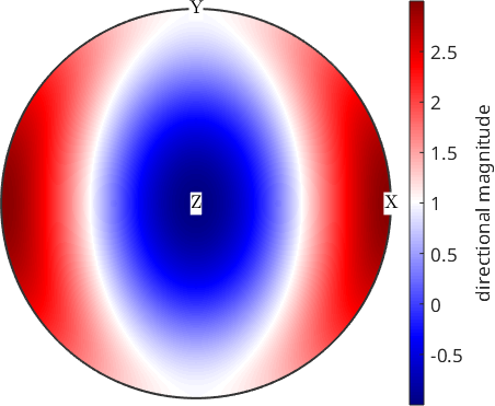

The labelled z, y, and x directions are the extrema of the coloured quadratic form. Their printed order matches the eigenvalues -1, 1, and 3. Negative values are colours here, not negative radii, so their sign remains visible.

Properties that depend on two directions

Not every tensor-derived quantity is a function of one direction. Poisson's ratio depends on a loading direction and a transverse direction. The transverse direction must be perpendicular to the loading direction.

Fix the loading direction p along z. The admissible transverse directions then form the great circle normal to p, so plotSection is the natural display.

p = vector3d.Z;
nu = C.PoissonRatio(p);

plotSection(nu,p,'color','interp','linewidth',5);
axis off;
mtexColorbar('title','Poisson''s ratio');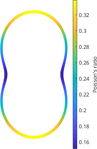

The closed curve is only the admissible great circle, not the whole sphere. Its changing radius and colour show that the transverse response varies as the transverse direction turns around z. Anisotropic Elasticity develops Poisson's ratio, shear modulus, and Young's modulus from the compliance tensor.

Specialized plots

Physical tensor classes provide plots tailored to the property they represent. Wave Velocities plots elastic-wave speed and polarization. Birefringence plots the optical response, and Piezo Electricity plots a signed third-rank response.

Continue with Tensor Averages to combine a single-crystal tensor with measured orientations or an ODF.

The maths behind directional magnitude

For a rank-\(r\) tensor \(T\), MTEX contracts the same unit direction into every tensor slot:

\[ Q(\vec x) = T_{i_1 \ldots i_r}\, x_{i_1} \cdots x_{i_r}, \qquad \vec x = 1. \]

This produces an S2Fun. Even-rank tensors satisfy \(Q(-\vec x)=Q(\vec x)\), while odd-rank tensors reverse sign.

Repeating the same direction also means that Q contains only the fully symmetric part of a general tensor. It is therefore a useful view, but it cannot encode every component of a higher-rank tensor.

Further reading

setMTEXpref('defaultColorMap',WhiteJetColorMap);