Elasticity

Elasticity is the reversible part of deformation. Apply a load and the material changes shape; remove the load and it returns. Strain measures that relative change in shape, while stress measures force per unit area. For small strains, the stiffness tensor maps strain linearly to stress.

A crystal generally responds differently in different directions, so its elastic behavior cannot be summarized by one modulus. The same directional stiffness controls how an elastic disturbance travels through the crystal. Elasticity therefore connects laboratory measurements of crystals to seismic observations of rocks.

A directional elastic response

The first example maps compressional-wave speed through an olivine crystal. It loads a stiffness tensor in GPa and attaches a density in \(\mathrm{g/cm}^3\).

plottingConvention.default('y↑→x');

cs = crystalSymmetry('mmm',[4.7646 10.2296 5.9942],...
  'mineral','Olivine');
C = stiffnessTensor.load( ...
  fullfile(mtexDataPath,'tensor','Olivine1997PC.GPa'),cs);

C = addOption(C,'density',3.355);

[vp,~,~] = velocity(C);
[vpMax,vpMaxDirection] = max(vp);
[vpMin,vpMinDirection] = min(vp);
vpRange = [vpMin,vpMax]

plot(vp,'complete','upper','noLabel')
mtexColorbar('title','v_p in km/s')
hold on
plot(vpMaxDirection(1),'Marker','s','MarkerEdgeColor','white',...
  'MarkerFaceColor','black')
plot(vpMinDirection(1),'Marker','o','MarkerEdgeColor','black',...
  'MarkerFaceColor','white')
hold off

vpRange =
    7.6533    9.7735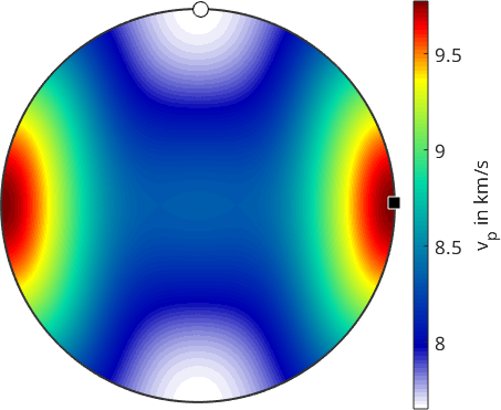

Red directions are fast and blue directions are slow. The black square marks the 9.77 km/s maximum, and the white circle marks the 7.65 km/s minimum. The maximum is 27.7% faster than the minimum, which is close to a thirty per cent contrast in a single crystal.

If flow aligns olivine grains in a rock, part of this anisotropy survives orientation averaging. The resulting directional contrast can influence a seismic signal measured hundreds of kilometres away.

Why density is required

It is common shorthand to say that a velocity is a stiffness divided by a density. More precisely, let \(L\) be the directional stiffness eigenvalue and let \(r\) be density. Their relation is \(v^2=L/r\), so squared speed, rather than speed, scales as stiffness divided by density.

A stiffness tensor carrying no density does not determine a physical wave speed. In that case MTEX warns and uses rho=1, so the returned values are not velocities in km/s. Storing the density on the tensor keeps every later velocity calculation consistent.

Three waves, not one

An isotropic solid supports two elastic wave types: one compressional mode and one shear speed with no preferred shear polarization. Elastic anisotropy splits the shear mode. A crystal consequently has three modes for each propagation direction: one quasi-compressional mode and two shear modes.

The three particle-motion directions are mutually perpendicular. Away from a symmetry direction, the quasi-compressional polarization need not be exactly parallel to propagation. The two shear modes also generally travel at different speeds and have definite polarizations.

This shear-wave splitting is directly observable. A shear wave entering an aligned rock can leave as two pulses separated in time. Their delay and polarization constrain the anisotropy accumulated along the path and, together with mineral physics, the rock texture that produced it.

Route through this chapter

Isotropic Theory begins with the familiar direction-independent case. It defines the usual elastic moduli and gives the reference against which anisotropic results are compared.

Anisotropic Theory introduces Hooke's law with the full tensor. It then computes directional Young's modulus, linear compressibility, Poisson's ratio, and shear modulus.

Wave Velocities solves the Christoffel equation for the three wave modes. It makes their speeds, polarizations, and splitting quantitative.

CPO Seismic Properties completes the workflow. It combines measured orientations, phase proportions, stiffness tensors, and densities into the seismic anisotropy of an aggregate.

Related chapters

Tensors develops the tensor operations and averaging schemes used here. ODFs and EBSD supply the crystal-orientation data required by aggregate averages. Deformation that is not recovered on unloading is treated in Plasticity.

References

Next

Continue with Isotropic Theory to learn how two elastic moduli describe a direction-independent material and how MTEX obtains an isotropic aggregate from randomly oriented crystals.

References

- E. H. Abramson, J. M. Brown, L. J. Slutsky, and J. Zaug, The elastic constants of San Carlos olivine to 17 GPa, Journal of Geophysical Research 102 (1997), 12253-12263, supplies the olivine stiffness tensor used in the example.
- J. F. Nye, Physical Properties of Crystals: Their Representation by Tensors and Matrices, Oxford University Press, 1985, develops the tensor description of elastic anisotropy and its dependence on direction.
- D. Mainprice, R. Hielscher, and H. Schaeben, Calculating anisotropic physical properties from texture data using the MTEX open-source package, Geological Society, London, Special Publications 360 (2011), 175-192, connects crystal orientations to aggregate elastic and seismic properties.