EBSD

Electron backscatter diffraction (EBSD) measures crystal orientation at points on a polished specimen surface. The indexing algorithm compares the diffraction pattern with candidate phases. It assigns a phase and an orientation at each point. Moving the beam across a scan lattice produces a map: a list of orientations tied to positions on the specimen.

This spatial link distinguishes an EBSD map from a bulk diffraction pole figure. A pole figure reports which orientations occur in a sampled volume. An EBSD map reports which orientation was assigned where on the measured surface. Grain size, neighbourhood, intragranular gradients, and boundary traces all depend on that where.

The plotting convention below draws specimen Y upward and specimen X to the right. It changes the screen layout, not the measured data.

plottingConvention.default('y↑→x');
mtexdata forsterite

ebsd = EBSDsquare (y↑→x, row↑→col)
 
 Phase  Orientations     Mineral         Color  Symmetry  Crystal reference frame
     0   58485 (24%)  notIndexed          none                                   
     1  152345 (62%)  Forsterite  LightSkyBlue       mmm                         
     2   26058 (11%)   Enstatite  DarkSeaGreen       mmm                         
     3   9064 (3.7%)    Diopside     Goldenrod     12/m1        X||a*, Y||b, Z||c
 
 Properties: bands, bc, bs, error, mad, oldId
 Scan unit : um
 X × Y × Z : [0 → 36550] × [0 → 16750] × [0 → 0]
 Normal vector: (0,0,1)
 Square grid  :336 × 732

Read the displayed EBSD summary as an inventory. It identifies the scan lattice and extent. It also lists the phases, the notIndexed measurements, and the available per-pixel properties.

An EBSD variable is a list, not an image. Each entry carries a position, a phase, and an orientation. The entries form an image-like map only because their positions usually lie on a square or hexagonal scan lattice.

Seeing phase and orientation

The same measurements can answer different questions depending on what supplies the colour. The left panel colours every measurement by phase. The right panel retains the original orientation plot for Forsterite and colours it by the crystal direction parallel to specimen Z.

newMtexFigure('layout',[1,2],'figSize','large');
plot(ebsd,'micronbar','off');
mtexTitle('phases');

nextAxis;
fo = ebsd('Forsterite');
plot(fo,fo.orientations,'ipfDirection',zvector,'micronbar','off');
mtexTitle('Forsterite orientations');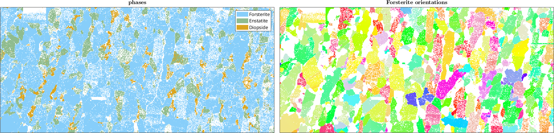

In the phase map, contiguous areas of the same colour show where each indexed phase occurs, while the white speckle is notIndexed. The broad colour domains in the orientation map are spatially coherent orientations within Forsterite. White now also includes every other phase, because only the Forsterite selection was plotted.

Orientation colour is not a measurement. An orientation colour key is a rule for turning a three-parameter orientation into three RGB values. Different keys can make the same orientations look different, and colour alone is not a quantitative orientation scale.

Recorded, missing, and derived data

A notIndexed entry is a recorded measurement whose diffraction pattern could not be indexed. It is a phase value, not an absent scan position. A band of notIndexed measurements along a boundary may therefore carry information about pattern overlap or specimen quality. Points outside the scanned region are absent from the list. So are lattice sites at which no measurement was retained.

Selecting one phase removes the other entries from the list; it does not replace them with blank pixels. The remaining positions can therefore have gaps. An operation that needs neighbours must recover the scan lattice, either internally or through an explicit gridding step.

Grains and orientation distributions are derived from this measurement list. A grain is a phase-homogeneous, spatially connected region of EBSD pixels produced by segmentation. Its outline depends on the segmentation rule; it is not a boundary measured directly by the detector. An orientation distribution function (ODF) discards position. It estimates a continuous density over orientation space.

These distinctions determine what a number means. On an equally spaced map, a pixel fraction measures surface area. It is not automatically a bulk specimen volume fraction. Step size, phase selection, and indexing quality can change a downstream result. So can filling, denoising, and grain segmentation.

Check the reference frame before analysis

A reference frame is the coordinate system in which data are expressed. EBSD positions describe how the stage moved, while the Euler angles encode orientations in a specimen frame. The two frames need not arrive aligned. Vendors and software versions use different conventions, and a file may not record the relationship completely.

The failure is quiet. A map with the wrong relationship still plots, reconstructs into grains, and produces pole figures. The results are rotated or mirrored. The numerical values alone do not expose the mistake. Read Reference Frame Alignment for your own data before trusting any downstream result.

Recommended reading order

Begin with Import, then check Reference Frame Alignment. Also review Orientations if the crystal-to-specimen map is new to you.

Continue with Plotting EBSD Maps and IPF Maps. The first explains the plot(where,what) pattern; the second explains the colour key used above. Then read Select, Select by Index, and Square and Hex Grids. The first two cut a map down - by phase, by region, by property, by condition - and most real analysis starts with one of these. Together the three pages establish phase, logical, positional, list, identifier, row-column, and lattice indexing. Learn those distinctions before using neighbour-based operations.

Orientation Plots then shows pole figures, inverse pole figures, sections, and orientation-space views of a selection. Grain Reconstruction turns measurements into grains and is the gateway to Grains.

After that foundation, choose the branch that matches the question.

Simulation creates maps with known answers for testing a processing chain. HDF5 Interface is a developer guide for vendor JSON configurations, while Export explains what different output formats preserve.

Further reading

Next

Grains and Grain Boundaries develop the regions and boundary network obtained by segmentation. A grain boundary in MTEX is a segment between neighbouring EBSD pixels assigned to different grains. It is derived from the map, not measured as a separate detector signal.

3D EBSD extends spatial analysis from a surface to a volume. Orientations develops the orientation geometry itself, and ODF develops continuous orientation distributions.