The Index of EBSD data

The Index of EBSD data edit page

In previous chapters we have discussed how to select EBSD data by properties. In this chapter we discus the ordering of EBSD pixels within MTEX. Lets start by importing some sample data

mtexdata twins

ebsd = EBSD (y↑→x)
 
 Phase  Orientations     Mineral         Color  Symmetry  Crystal reference frame
     0     46 (0.2%)  notIndexed                                                 
     1  22833 (100%)   Magnesium  LightSkyBlue     6/mmm       X||a*, Y||b, Z||c*
 
 Properties: bands, bc, bs, error, mad
 Scan unit : um
 X x Y x Z : [0, 50] x [0, 41] x [0, 0]
 Normal vector: (0,0,1)

and restricting it to very small rectangular subset

poly = [44 0 4 2];
ebsd = ebsd(inpolygon(ebsd,poly));

plot(ebsd,ebsd.orientations,'micronbar','off','edgecolor','k')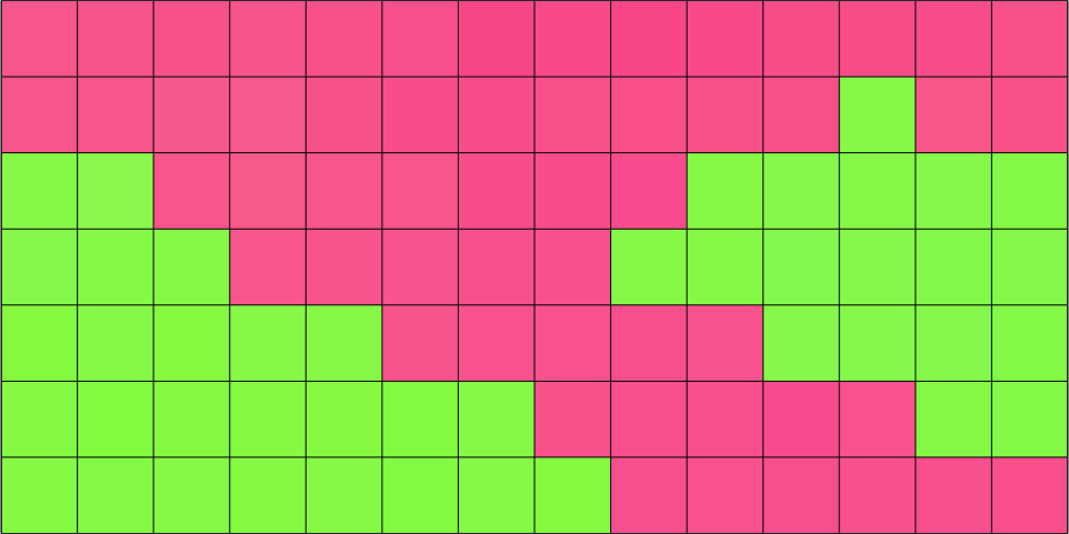

In the above plot each square corresponds to one entry in the variable ebsd which as an index from 1 to 98. Let us visualize this index

text(ebsd,1:length(ebsd))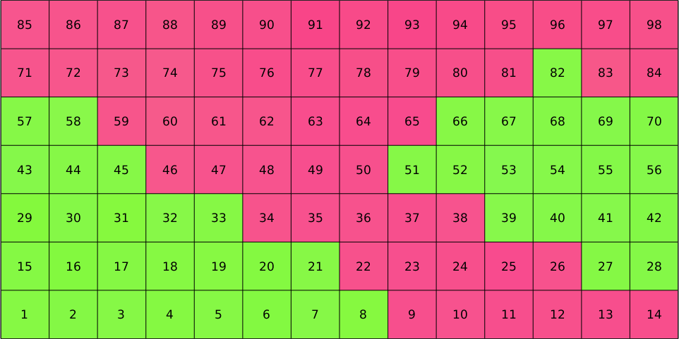

We may easily select specific pixels by specifying their indices

hold on
plot(ebsd(16:18),'edgeColor','red','facecolor','none','linewidth',4)
legend off
hold off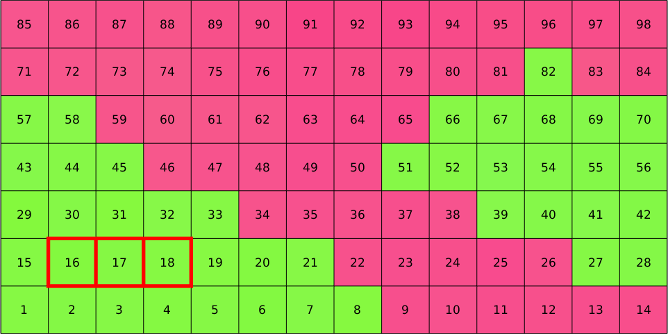

Whether lines or columns run first is not related to MTEX but inherits from the ordering of the imported EBSD data. Since, we have restricted our large EBSD map to the small subset the indices of restricted data does not coincide with the indices of the imported data anymore. However, the original indices are still stored in ebsd.id. Lets visualize those

plot(ebsd,ebsd.orientations,'micronbar','off','edgecolor','k')
text(ebsd,ebsd.id)

In order to select EBSD data according to their original id use the option 'id', i.e.,

hold on
plot(ebsd('id',316:318),'edgeColor','red','facecolor','none','linewidth',4)
legend off
hold off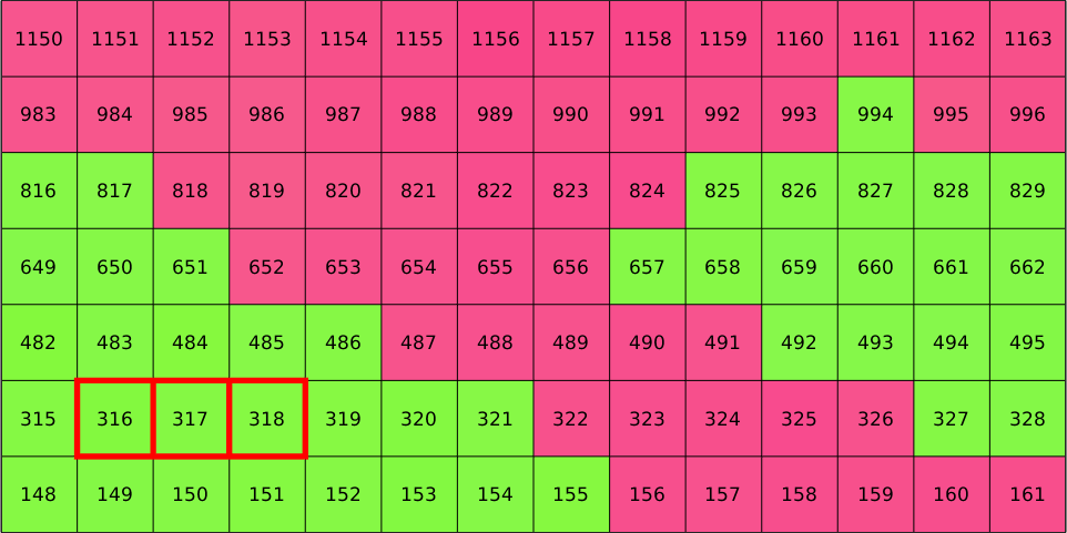

Square Grids

In the cases of gridded data it is often useful to convert them into a matrix form.

ebsd = ebsd.gridify;

plot(ebsd,ebsd.orientations,'micronbar','off')

[i,j] = ndgrid(1:size(ebsd,1),1:size(ebsd,2));
str = arrayfun(@(a,b) ['(' int2str(a) ',' int2str(b) ')'],i,j,'UniformOutput',false);
text(ebsd,str)

This allows to select EBSD data simply by their coordinates within the grid, e.g., by

hold on
plot(ebsd(2,2:4),'edgeColor','red','facecolor','none','linewidth',4)
legend off
hold off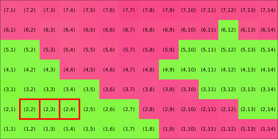

Note that the gridify command changes the order of measurements. They are now sorted such that rows runs first and columns second, as this is the default convention how Matlab indexes matrices.

plot(ebsd,ebsd.orientations,'micronbar','off')
text(ebsd,1:length(ebsd))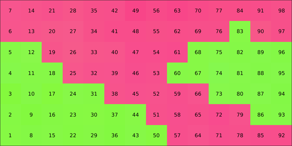

Hexagonal Grid

The command gridify may also be applied to EBSD data measured on a hexagonal grid.

mtexdata titanium silent

ebsd = ebsd.gridify

ebsd = EBSDhex (y↑→x)
 
 Phase  Orientations           Mineral         Color  Symmetry  Crystal reference frame
     0    8100 (99%)  Titanium (Alpha)  LightSkyBlue       622       X||a, Y||b*, Z||c*
 
 Properties: ci, grainid, iq, sem_signal, oldId
 Scan unit : um
 X x Y x Z : [0, 1002] x [0, 998] x [0, 0]
 Normal vector: (0,0,1)
 Hex grid     :97 x 84

This rearranges the measurements in a matrix form which can be indexed similarly as in the square case.

ebsd = ebsd(10:16,68:79);

Lets visualize the matrix coordinates for the hexagonal grid

plot(ebsd,ebsd.orientations,'edgeColor','k','micronbar','off')
axis off

[i,j] = ndgrid(1:size(ebsd,1),1:size(ebsd,2));
str = arrayfun(@(a,b) ['(' int2str(a) ',' int2str(b) ')'],i,j,'UniformOutput',false);
text(ebsd,str)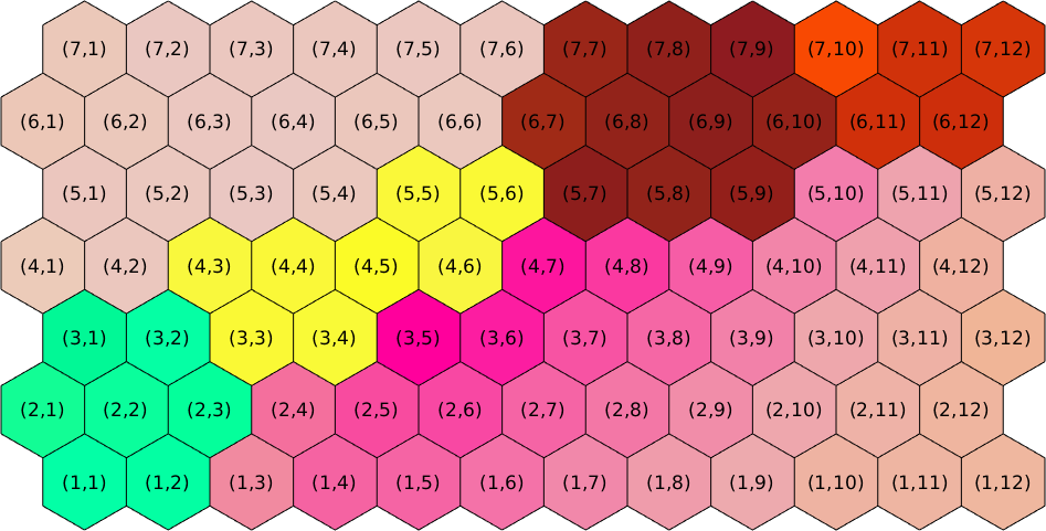

Cube Coordinates

In hexagonal grids it is sometimes advantageous to use three digit cube coordinates to index the cell. This can be done using the commands hex2cube and cube2hex. Much more details on indexing hex grids can be found at here.

plot(ebsd,ebsd.orientations,'edgeColor','k','micronbar','off')
axis off

[i,j] = ndgrid(1:size(ebsd,1),1:size(ebsd,2));
[x,y,z] = ebsd.hex2cube(i,j);
str = arrayfun(@(a,b,c) ['(' int2str(a) ',' int2str(b) ',' int2str(c) ')'],x,y,z,'UniformOutput',false);
text(ebsd,str)