The orientation distribution function (ODF), sometimes also called orientation density function, is a function on the orientation space that associates to each orientation \(g\) the volume percentage of crystals in a polycrystaline specimen that are in this specific orientation. Formaly, this is often expressed by the formula
\[\mathrm{odf}(g) = \frac{1}{V} \frac{\mathrm{d}V(g)}{\mathrm{d}g}.\]
Let us demonstrate the concept of an ODF at the example of an Titanium alloy. Using EBSD crystal orientations \(g_j\) have been measured at a hexagonal grid \((x_j,y_j)\) on the surface of the specimen. We may visualize these orientations by plotting accordingly rotated crystal shapes at the positions \((x_j,y_j)\).
% import the data
mtexdata titanium

% define the habitus of titanium as a somple hexagonal prism
cS = crystalShape.hex(ebsd.CS);

% plot colored orientations
plot(ebsd,ebsd.orientations,'micronbar','off')

% and on top the orientations represented by rotated hexagonal prism
hold on
plot(reduce(ebsd,4),40*cS)
hold off
ebsd = EBSD (y↑→x)
Phase Orientations Mineral Color Symmetry Crystal reference frame
0 8100 (100%) Titanium (Alpha) LightSkyBlue 622 X||a, Y||b*, Z||c*
Properties: ci, grainid, iq, sem_signal
Scan unit : um
X x Y x Z : [0, 996] x [0, 998] x [0, 0]
Normal vector: (0,0,1)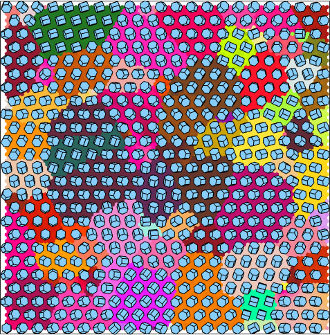
The idea of the orientation distribution function is to forget about the spatial coordinates \((x_j,y_j)\) and consider the orientations as points in the three dimensional orientation space.
plot(ebsd.orientations,'Euler')plot 2000 random orientations out of 8100 given orientations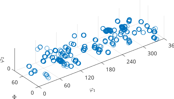
As the orientation space is not an Euclidean one there is no canonical way of visualizing it. In the above figure orientations are represented by its three Euler angles \((\varphi_1, \Phi, \varphi_2)\). Other visualizations are discussed in the section 3D Plots. The orientation distribution function is now the relative frequency of the above points per volume element and can be computed by the command calcDensity.
odf = calcDensity(ebsd.orientations)odf = SO3FunHarmonic (Titanium (Alpha) → y↑→x)
bandwidth: 25
weight: 1More detais about the computation of a density function from discrete measurements can be found in the section Density Estimation.
The resulting orientation distribution function odf can be evaluated for any arbitrary orientation. Lets us e.g. consider the orientation
ori = orientation.byEuler(0,0,0,ebsd.CS);Then value of the ODF at this orientation is
odf.eval(ori)ans =
0.8166The resulting value needs to be interpreted as multiple of random distribution (mrd). This means that for the specimen under investigation it is less likely to have a crystal with orientation (0,0,0) compared to a completely untextured specimen which has a constant orientation distribution function that is equal to \(1\) everywhere.
Since, an ODF can be evaluated at any point in the orientation space we may visualize it as a contour plot in 3d
plot3d(odf,'Euler')
hold on
plot(ebsd.orientations,'Euler','MarkerEdgeColor','k')
hold off
plot 2000 random orientations out of 8100 given orientations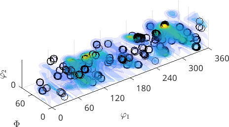
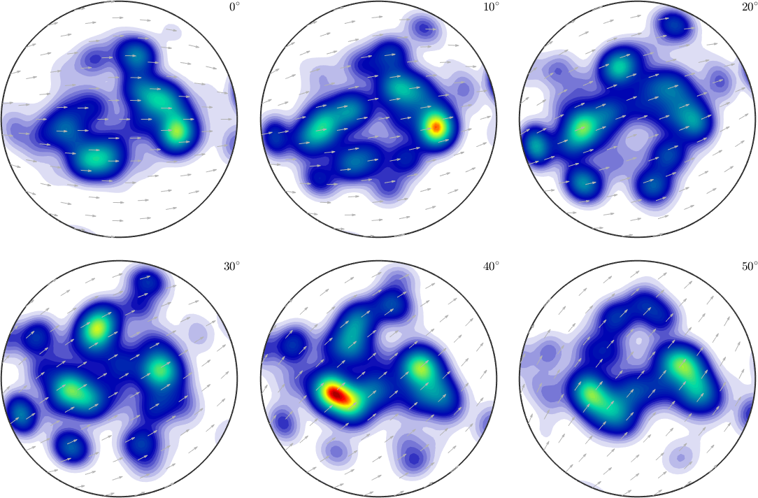
Three dimensional plots of an ODF in Euler angle space are for various reason not very recommended. A geometrically much more reasonable representation are so-called sigma sections.
plotSection(odf,'sigma')