Transparency

Transparency reveals information that an opaque object would cover. Use it to expose overlapping markers, combine complementary maps, or look through a three-dimensional surface.

An alpha value controls how strongly a plotted object covers the objects behind it. An alpha value of 0 is completely transparent. A value of 1 is completely opaque. MTEX uses different option names for different objects:

Each option accepts values in the interval \([0,1]\). Transparency requires the 'opengl' figure renderer, which is MATLAB's default.

Reveal overlapping markers

Start with 2000 orientations concentrated around the identity orientation. Project the same sample onto three pole figures, one for each crystal direction.

cs = crystalSymmetry('m-3m');
odf = unimodalODF(orientation.id(cs),'halfwidth',10*degree);
ori = odf.discreteSample(2000);

h = Miller({1,0,0},{1,1,0},{1,1,1},cs);

Opaque markers cover one another. The concentrated orientations appear as solid blobs. Neither the number of points nor the shape of each maximum is easy to judge.

plotPDF(ori,h,'MarkerSize',5,'all')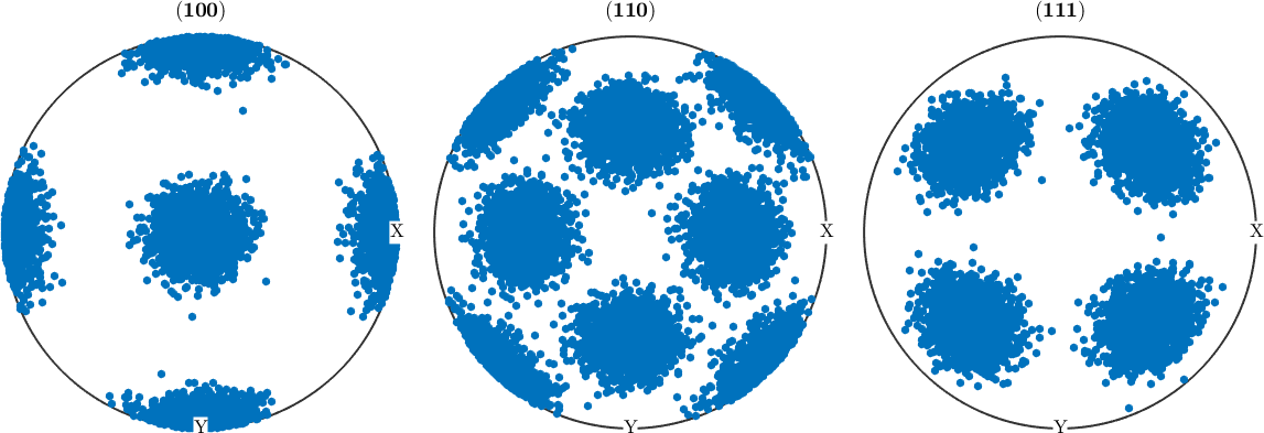

Set 'MarkerAlpha' to make both the marker faces and edges almost transparent. Repeated overlap stays dark, whereas isolated orientations become faint. The result resembles a density plot.

plotPDF(ori,h,'MarkerAlpha',0.05,'MarkerSize',5,'all')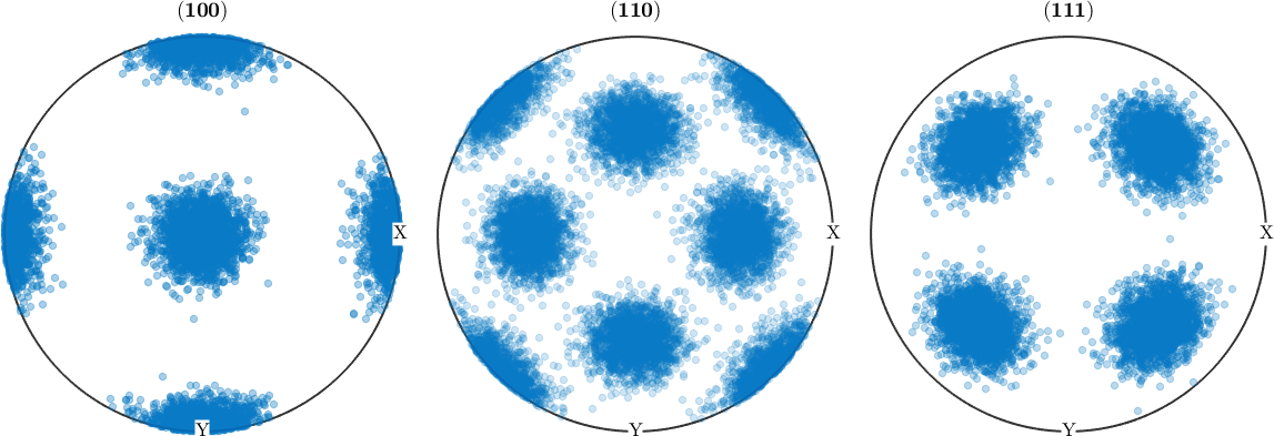

Marker faces and edges can instead have separate alpha values. The edges of overlapping markers accumulate faster than their faces. Keeping the edges slightly more opaque can reveal individual markers without filling a maximum completely. In the fringes the rings resolve; the cores of the strongest maxima still saturate.

plotPDF(ori,h,'MarkerFaceAlpha',0.01,'MarkerEdgeAlpha',0.05,...
  'MarkerSize',10,'all')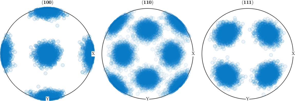

Transparency gives only a visual approximation of point density. Compute a kernel density estimate when the density itself matters. The final plot shows that estimate as filled contours. Density Estimation explains how MTEX computes it.

plotPDF(ori,h,'contourf')
mtexColorbar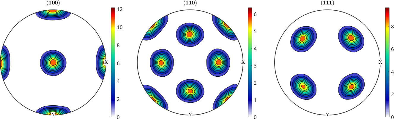

Superpose EBSD maps

A common use of transparency is to superpose two EBSD maps. Here band contrast supplies a greyscale background. A half-transparent orientation map supplies the crystallographic colour.

plottingConvention.default('y↑→x');
mtexdata forsterite silent

plot(ebsd,ebsd.bc)
mtexColorMap black2white

hold on
plot(ebsd('Forsterite'),ebsd('Forsterite').orientations,'faceAlpha',0.5)
hold off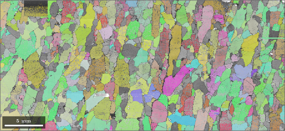

The result shows orientation and measurement quality at the same time. Dark structure from the band-contrast map remains visible beneath the orientation colours. IPF Maps explains how a colour key assigns those colours to orientations.

Make transparency depend on a property

A per-pixel property stores one value for every EBSD measurement. 'faceAlpha' can accept those values and make each map cell independently transparent. This example divides band contrast by its mean and clips the result at 1. Every alpha value therefore remains in the valid interval.

ebsdF = ebsd('Forsterite');

alpha = min(ebsdF.bc ./ mean(ebsdF.bc), 1);

plot(ebsdF,ebsdF.orientations,'faceAlpha',alpha,'figSize','large')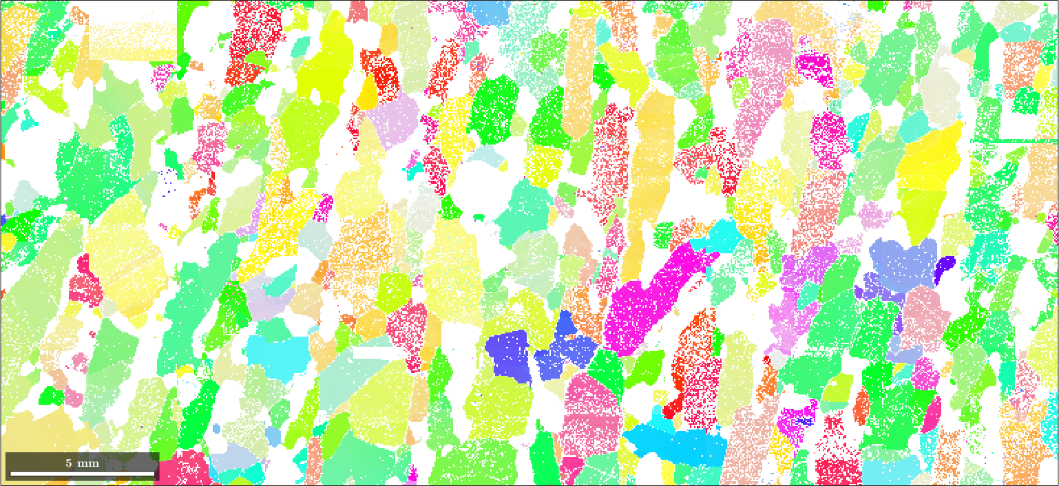

Low-band-contrast pixels fade while pixels at or above the mean remain opaque. Pixels near grain boundaries often fade because overlapping Kikuchi patterns from two grains tend to lower the band contrast there. Local misorientation is another useful alpha value. See Grain Reference Orientation Deviation for that construction.

Superpose a grain map

Grain maps use the same 'faceAlpha' option. MTEX also weights a grain's transparency by its colour. Light-coloured grains consequently become more transparent than dark-coloured grains. The 'translucent' option is a synonym for 'faceAlpha'.

grains = calcGrains(ebsd('indexed'),'angle',10*degree);
grains = smoothBoundary(grains,5);

plot(ebsd,ebsd.bc)
mtexColorMap black2white

hold on
plot(grains('Forsterite'),grains('Forsterite').meanOrientation,...
  'faceAlpha',0.5)
hold off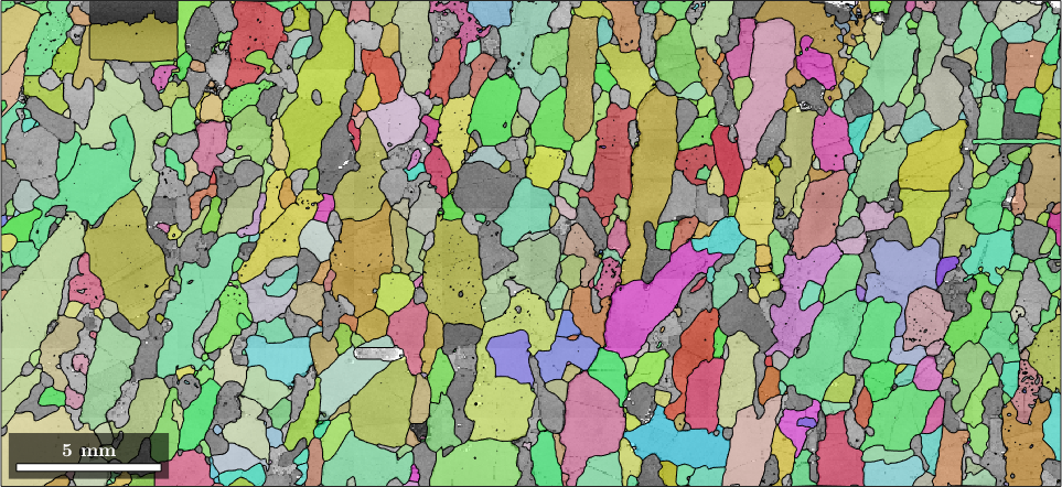

The greyscale map supplies the variation within each grain. The transparent grain colours summarize the mean orientation of each forsterite grain. Compare the fine background structure with the piecewise-constant colour of the grain layer.

Fade low-angle grain boundaries

Line plots such as grain boundaries use 'edgeAlpha'. It accepts one value for the whole plot or one value for each boundary segment. Here the alpha increases with misorientation angle and reaches full opacity at 30 degrees. The call to min keeps larger angles at the valid maximum.

gB = grains.boundary('Forsterite','Forsterite');
boundaryAlpha = min(gB.misorientation.angle ./ (30*degree),1);

plot(grains,'translucent',0.5,'micronbar','off')
legend off

hold on
plot(gB,'edgeAlpha',boundaryAlpha,'lineWidth',3)
hold off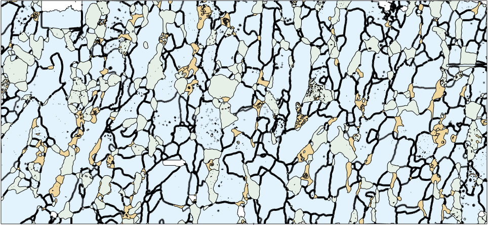

Every segment here is at least as strong as the 10 degree segmentation angle that created it, and four fifths are at or above 30 degrees, so the network is drawn almost uniformly opaque. The mechanism is what matters: an alpha vector fades each segment by its own misorientation, and on a map segmented at a lower angle the weakest boundaries would nearly disappear.

Look through transparent surfaces

Transparency also reveals the inside of a three-dimensional object. A transparent olivine crystal shape shows its back faces through the front faces.

cS = crystalShape.olivine;

plot(cS,'faceAlpha',0.2)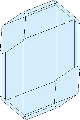

The same device becomes more useful when the crystal contains another object. In this cubic example, transparency keeps the slip-system geometry visible without hiding the crystal outline.

sS = slipSystem.fcc(crystalSymmetry('432'));
cSfcc = crystalShape.cube(crystalSymmetry('432'));

plot(cSfcc,'faceAlpha',0.2)
hold on
plot(cSfcc,sS(1),'faceColor','blue','faceAlpha',0.5)
hold off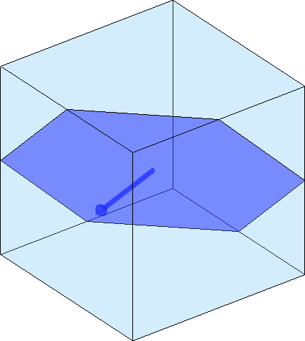

Three-dimensional ODF plots apply transparency automatically. A contour level becomes more opaque as its value increases. Maxima therefore remain visible through lower-valued outer levels. See Visualizing ODFs for the available three-dimensional plots.

close all
plot3d(SantaFe)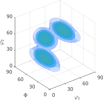

Export figures that contain transparency

Transparency is a feature of the 'opengl' renderer. A figure containing transparent objects cannot be exported as true vector graphics. During PDF or EPS export, MATLAB either rasterizes the figure or drops its transparency. Export such a figure as a bitmap instead, for example:

saveFigure('transparency.png')

See Exporting Figures for format and resolution choices.

References