Grain Orientation Parameters

Grain Orientation Parameters edit page

In this section we discuss properties of grains that are related to the distribution of orientations within the grains, i.e.,

`meanOrientation`	mean orientation	`GOS`	grain orientation spread
`GAM`	grain average misorientation	`GAX`	grain average misorientation axis

As usual, we start by importing some EBSD data and computing grains

close all; plotx2east

% import the data
mtexdata ferrite silent

% compute grains
[grains, ebsd.grainId] = calcGrains(ebsd('indexed'));
ebsd(grains(grains.grainSize < 5)) = [];
[grains, ebsd.grainId] = calcGrains(ebsd('indexed'),'threshold',7.5*degree);
ebsd = ebsd.project2FundamentalRegion;
grains = smooth(grains,5);

% plot the data
plot(ebsd, ebsd.orientations)
hold on
plot(grains.boundary,'lineWidth',2)
hold off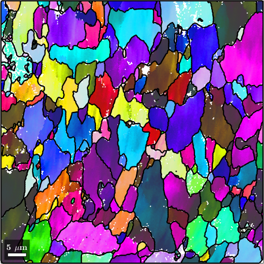

Grain average orientation

As by construction grains consist of pixels with similar orientation. In order to access all the orientations that belong to a specific grain we make use of the property ebsd.grainId where we have stored during grain reconstruction for every EBSD pixel to which grain it belongs. Hence, we may use logical indexing on our EBSD variable ebsd to find all orientations that belong to a certain grainId.

% select a grain by x and y coordinates
grainSel = grains(42,17)

% all EBSD orientations within the grain
ori = ebsd(grainSel).orientations

grainSel = grain2d
 
 Phase  Grains  Pixels  Mineral  Symmetry  Crystal reference frame
     0       1    1949  Ferrite       432                         
 
 boundary segments: 363 (64 µm)
 inner boundary segments: 0 (0 µm)
 triple points: 15
 
  Id   Phase   Pixels   phi1   Phi   phi2         GOS
 235       0     1949    144    41    301   0.0434024
 
 
ori = orientation (Ferrite → xyz)
  size: 1949 x 1

We could now use the command mean to compute the grain average orientation from these individual orientations. A more direct approach, however, is to access the property grain.meanOrientation which has been filled with the mean orientations during grain reconstruction.

plot(grains, grains.meanOrientation)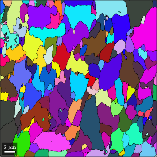

Misorientation to the grain mean orientation

Once we have a reference orientation for each grain - the grain meanorientation ori_ref - we may want to analyze the deviation of the individual orientations within the grain from this reference orientation. The grain reference orientation deviation (GROD) is the misorientation between each pixel orientation to the grain mean orientation defined as

mis2mean = inv(grainSel.meanOrientation) .* ori

mis2mean = misorientation (Ferrite → Ferrite)
  size: 1949 x 1

While the above command computes the misorientations to the grain mean orientation just for one grain the command calcGrod computes it for all grains simultaneously

mis2mean = calcGROD(ebsd, grains)

mis2mean = misorientation (Ferrite → Ferrite)
  size: 58967 x 1

Grain orientation spread (GOS)

The full misorientation to the mean orientation is often not so simple to understand. A good starting point is to just look at the misorientation angles to the grain mean orientation. The average of the misorientation angles to the grain mean orientation is called grain orientation spread (GOS) and can be computed by the command grainMean which averages arbitrary EBSD properties over grains. Here, we use it to average the misorientation angle for each grain separately.

% take the average of the misorientation angles for each grain
GOS = ebsd.grainMean(mis2mean.angle, grains);

% plot it
plot(grains, GOS ./ degree)
mtexColorbar('title','GOS in degree')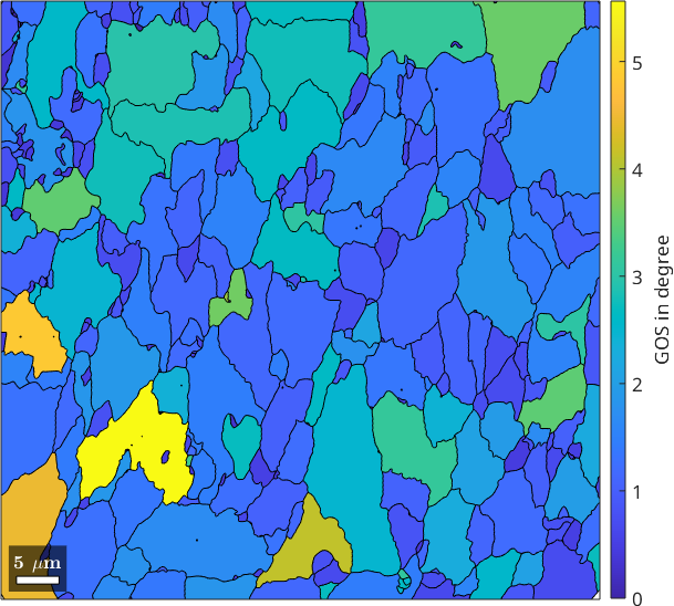

It should be noted that the GOS is also directly available as the grain property grains.GOS.

The function grainMean can also be used to compute the maximum misorientation angle to the mean orientation within each grain. To achieve this we have to pass the function @max as an additional argument. Note, that you can replace this function also with any other statistics like the median, or some quantile.

% compute the maximum misorientation angles for each grain
MGOS = ebsd.grainMean(mis2mean.angle, grains, @max);

% plot it
plot(grains, MGOS ./ degree)
mtexColorbar('title','MGOS in degree')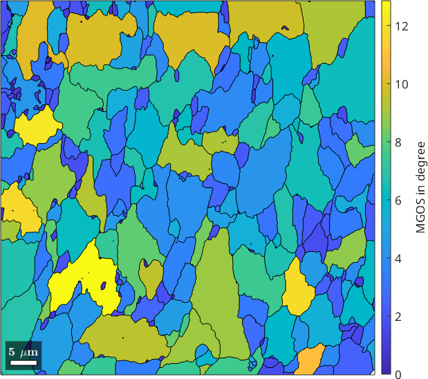

Grain average misorientation (GAM)

A measure that is often confused with the grain orientation spread is the grain average misorientation (GAM). The GAM is defined as the kernel average misorientation (KAM) averaged over each grain. Hence, we can compute is by using the functions ebsd.KAM and grainMean.

gam = ebsd.grainMean(ebsd.KAM, grains);

plot(grains,gam./degree)
mtexColorbar('title','GAM in degree')
setColorRange([0,3])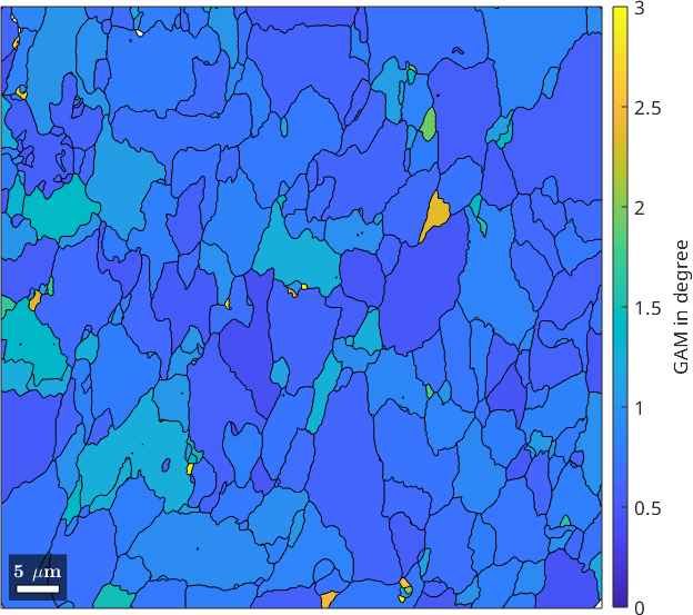

While the GOS measures global orientation gradients within a grain the GAM reflect the average local gradient.

The misorientation axis (crystal dispersion axis)

Under certain conditions, deformation may result in the dispersion of orientations within a grain. This can usually be the case when deformation is accommodated by slip on one dominant slip system for each grain and conditions are such, that the resulting orientation gradients are preserved in the material (as it is the case in many geomaterials deforming at moderate temperatures). In such a case, we would expect the orientations inside a grain to be aligned along a line with a specific misorientation axis to the mean orientation. Such a line is called fibre and we can use the command fibre.fit to find the best fitting fibre for a given list of orientations. Lets do this for a single grain.

% visualize the orientations within the selected  grain in a pole figure
figure(2)
h = Miller({1,0,0},ebsd.CS);
plotPDF(ebsd(grainSel).orientations,h,'MarkerSize',2,'all')

% fit a fibre to the orientations within the grain
[f,lambda,fit] = fibre.fit(ebsd(grainSel).orientations,'local');

% add the fibre to the pole figure
hold on
plotPDF(f.symmetrise,h,'lineColor','orange','linewidth',2)
hold off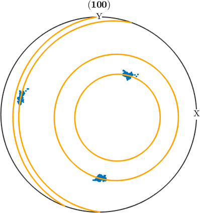

The function fibre.fit has three output arguments. The first one f is the fitted fibre. From this we can easily detect the prominent misorientation axis in specimen coordinates by f.r and in crystal coordinates by f.h.

f.r
f.h

% We can see that the dispersion of directions is minimal for those
% parallel to |f.r| respectively |f.h|.
hold on
plot(ebsd(grainSel).orientations.*f.h,'MarkerSize',2,'all','MarkerFaceColor','k','antipodal')
hold off

ans = vector3d
          x         y         z
  -0.281993 0.0471325 -0.958258
 
ans = Miller (Ferrite)
       h       k       l
  1.6922 -0.1497 -2.3132

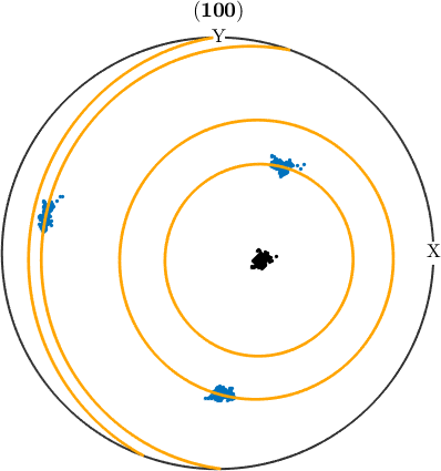
The second output argument lambda are the eigenvalues of the orientation matrix. The largest eigenvalue indicates are localized the orientations are. The second largest eigenvalue is a measure how much the orientation distributed along the fitted fibre. The third and forth eigenvalue describe how much the orientations scatter off the fibre. The scatter off the fibre is more conveniently described in the last output argument fit, which is the mean misorientation angle of the orientations to the fitted fibre.

lambda

fit./degree

lambda =
    0.0001    0.0001    0.0004    0.9994
ans =
    0.0329

Lets perform the above analysis for all large grains

grainsLarge = grains(grains.grainSize > 50);

% loop through all grains
for k = 1:length(grainsLarge)

  % fit a fibre
  [f,lambda(k,:),fit(k)] = fibre.fit(ebsd(grainsLarge(k)).orientations,'local');

  % store the misorientation axes in crystal and specimen symmetry
  GAX_C(k) = f.h; %#ok<*SAGROW>
  GAX_S(k) = f.r;

end

And plot the fit, the third and the second largest eigenvalues. We clearly see how the fit is related to the third largest eigenvalue \(\lambda_2\).

plot(grainsLarge,lambda(:,3))
mtexTitle('\(\lambda_3\)')

nextAxis(1,2)
plot(grainsLarge,lambda(:,2))
mtexTitle('\(\lambda_2\)')

nextAxis(1,3)
plot(grainsLarge,fit./degree)
mtexTitle('fit')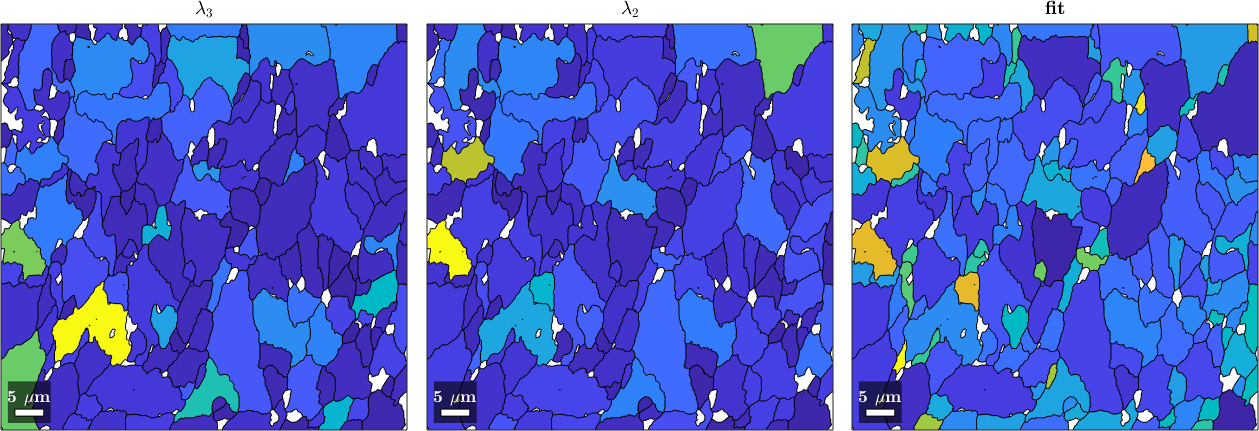

The crystal dispersion axes in crystal coordinates

In order to visualize the crystal dispersion axes we first need to define an appropriate color key for crystal directions. This can be done with the command HSVDirectionKey. Note, that we need to specify the option 'antipodal' since for the crystal dispersion axes we can not distinguish between antipodal directions.

% define the color key
cKey = HSVDirectionKey(ebsd.CS,'antipodal');

% plot the color key and on top the dispersion axes
plot(cKey)
hold on
plot(GAX_C.project2FundamentalRegion,'MarkerFaceColor','black')
hold off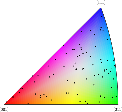

Now we can use this colorkey to visualize the misorientation axes in the grain map

% compute colors from the misorientation axes
color = cKey.direction2color(GAX_C);

% plot the colored grains
plot(grainsLarge, color)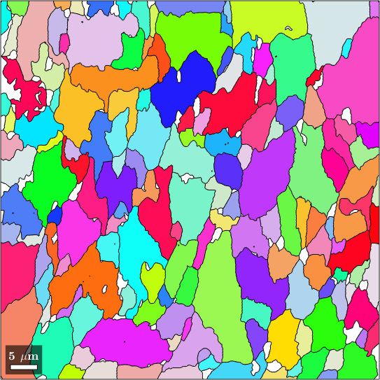

The crystal dispersion axes in specimen coordinates

Colorizing the crystal dispersion axes in specimen coordinates is unfortunately much more complicated. In fact, it is mathematically impossible to find a corresponding color key without color jumps. Instead MTEX visualizes axes in specimen coordinates by compass needles which are entirely gray if in the plane and get divided into black and white to indicate which end points out of the plane and which into the plane.

plot(grains, GOS./degree)
mtexColorbar('title','GOS in degree')

hold on
plot(grainsLarge, GAX_S)
hold off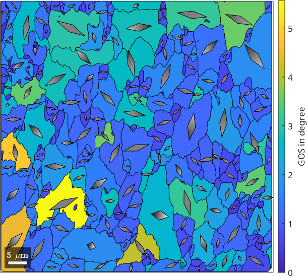

In many materials, a direct relation can be observed between the position of the crystal dispersion axis in specimen coordinates and the inferred type of flow. E.g. in many geomaterials which have undergone (close to) simple shear progressive deformation, the average of the crystal dispersion axes align parallel to the vorticity axis of flow; in pure shear progressive deformation, crystal dispersion axes form a girdle with a normal parallel to the shortening direction.

plot(GAX_S,'antipodal','MarkerSize',4)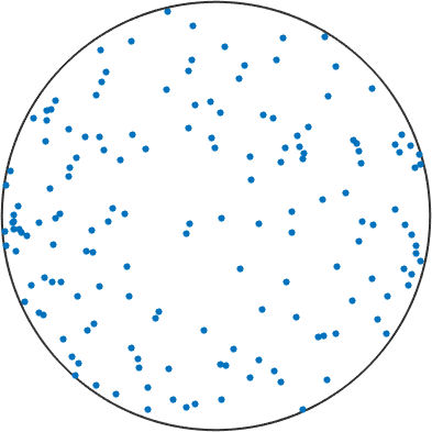

to get some idea about any preferred direction, we can add contours, weighted by the fit. grains with a large mean misorientation angle will also have a more well defined direction of the dispersion axis.

hold on
plot(GAX_S,'contour','antipodal','weights', fit,'contours',[1 2 3],'halfwidth',10*degree,'linewidth',2)
hold off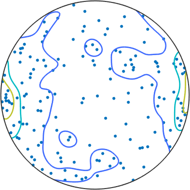

Here we do not see this clear of a picture (maybe because this is a piece of steel which might behave differently, maybe because we do not consider a large enough number of grains) Question: if this is processed steel, which sample directions is pointing to the east?

TODO: Testing on Bingham distribution for a single grain

Although the orientations of an individual grain are highly concentrated, they may vary in the shape. In particular, if the grain was deformed by some process, we are interested in quantifications.

%cs = ebsd(grains(id)).CS;
%ori = ebsd(grain_selected).orientations;
%plotPDF(ori,[Miller(0,0,1,cs),Miller(0,1,1,cs),Miller(1,1,1,cs)],'antipodal')

Testing on the distribution shows a gentle prolatness, nevertheless we would reject the hypothesis for some level of significance, since the distribution is highly concentrated and the numerical results vague.

% calcBinghamODF(ori,'approximated')

%T_spherical = bingham_test(ori,'spherical','approximated');
%T_prolate   = bingham_test(ori,'prolate',  'approximated');
%T_oblate    = bingham_test(ori,'oblate',   'approximated');

%[T_spherical T_prolate T_oblate]

%
%
%<html>
%   <div class="note">
%      <b>ok&lt;*NASGU&gt;
%</b>
%      <text/>
%   </div>
%</html>
%