Sachs Model

A polycrystal starts to yield when its grains start to slip. Predicting the required stress needs an assumption about how neighbouring grains constrain one another.

The Taylor model assumes that every grain undergoes the specimen strain. Enforcing that strain requires five independent slip systems per grain and gives an upper bound on strength. The calculation is introduced on the Taylor Model page.

The Sachs model makes the opposite assumption: every grain feels the same stress. Each grain slips on its best-oriented system without accommodating what its neighbours need. The grains therefore deform independently, the model specimen does not remain compatible, and the predicted strength is a lower bound.

MTEX has no calcSachs command because the construction needs only the Schmid factor. This page turns those single-crystal factors into a polycrystal bound and identifies the selected system.

Resolve the stress in every grain

Use the twelve geometric fcc slip systems and a uniaxial tension along specimen \(z\). The 'antipodal' option identifies the two shear senses of one system; the absolute Schmid factor below makes their activation equivalent.

cs = crystalSymmetry('m-3m');
sS = symmetrise(slipSystem.fcc(cs),'antipodal')

sigma = stressTensor.uniaxial(vector3d.Z)

sS = slipSystem (m3̅m)
 size: 12 × 1
 
   u    v    w  | h    k    l CRSS
   0    1   -1    1    1    1    1
  -1    0    1    1    1    1    1
   1   -1    0    1    1    1    1
   1   -1    0    1    1   -1    1
   1    0    1    1    1   -1    1
   0    1    1    1    1   -1    1
   0    1   -1   -1    1    1    1
   1    0    1   -1    1    1    1
   1    1    0   -1    1    1    1
  -1    0    1    1   -1    1    1
   1    1    0    1   -1    1    1
   0    1    1    1   -1    1    1
 
sigma = stressTensor (y↓→x)
  rank: 2 (3 × 3)
 
 0 0 0
 0 0 0
 0 0 1

Draw 10,000 orientations from a random texture.

ori = orientation.rand(10000,cs);

The stress is expressed in the specimen frame, whereas sS is expressed in the crystal frame. Applying the inverse orientation maps the same stress into each crystal frame before the Schmid factors are evaluated.

SF = sS.SchmidFactor(inv(ori) * sigma);

size(SF)

ans =
       10000          12

The result has one row per grain orientation and one column per geometric slip system. The Sachs assumption retains only the largest absolute factor in each row.

[SFmax,active] = max(abs(SF),[],2);

See how one system is selected

The bars are the twelve candidate factors for the first grain. The red marker is the maximum and therefore the system selected by the model.

bar(abs(SF(1,:)))
hold on
plot(active(1),SFmax(1),'or','MarkerFaceColor','r')
hold off
xlabel('slip-system index')
ylabel('absolute Schmid factor')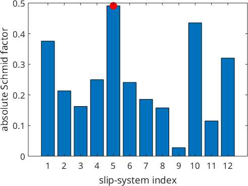

The plot makes the single-slip assumption visible: all smaller bars are discarded even though several systems may be similarly oriented. The selected index can be used to recover the actual crystallographic system.

sS(active(1))

ans = slipSystem (m3̅m)
 
  u    v    w  | h    k    l CRSS
  1    0    1    1    1   -1    1

Compute the Sachs factor

Let every system have the same critical resolved shear stress (CRSS) \(\tau_c\). Grain \(i\) begins to slip when its applied stress reaches \(\tau_c/m_i\), where \(m_i\) is its maximum Schmid factor. Averaging the normalized stresses gives the Sachs factor \(M_S\):

\[M_S = \frac{1}{N}\sum_{i=1}^{N}\frac{1}{m_i}. \]

MSachs = mean(1./SFmax)

MSachs =
    2.2340

The result is 2.24 for this random fcc texture, matching the classical random-texture value. Thus the Sachs model predicts a macroscopic stress of \(2.24\tau_c\).

Compare the lower and upper bounds

For comparison, evaluate the Taylor factor for 2,000 random orientations. The strain is volume preserving and represents uniaxial extension along specimen \(x\). Taylor decomposition needs both signed shear senses.

eps = strainTensor(diag([1 -0.5 -0.5]));
oriTaylor = orientation.rand(2000,cs);
sSTaylor = symmetrise(slipSystem.fcc(cs));
MTaylor = calcTaylor(inv(oriTaylor) * eps,sSTaylor);
mean(MTaylor)

ans =
    3.0499

The mean Taylor factor is 3.07, again the classical value. The two models bracket the truth: a real random fcc polycrystal yields between 2.24 and 3.07 times the common CRSS. Its position between the bounds depends on how strongly the grains constrain one another.

Inspect the distribution behind the mean

The average hides the orientation dependence. Every grain has its own best Schmid factor between zero and the theoretical maximum of 0.5.

histogram(SFmax,20)
xlabel('maximum absolute Schmid factor')
ylabel('number of orientations')

min(SFmax)

ans =
    0.2751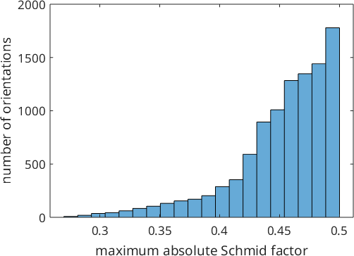

The distribution is strongly skewed towards 0.5. The smallest value in these 10,000 orientations rounds to 0.28. With twelve systems available, all of them are badly aligned only for a very particular orientation.

The vector active records which system was chosen in every grain. A Sachs calculation therefore predicts which slip trace should appear in the microscope. That prediction can be checked directly, unlike the idealized yield-stress bound itself.

References

Next

The Sachs bound selects one system independently in each grain. Continue with Single Slip Model to follow the texture that develops when one prescribed system supplies the crystallographic spin.

References

- U. F. Kocks, C. N. Tomé and H.-R. Wenk, Texture and Anisotropy, Cambridge University Press, 1998, derives the Sachs and Taylor bounds and gives their classical random-texture values.
- H. J. Bunge, Some Applications of the Taylor Theory of Polycrystal Plasticity, Kristall und Technik 5 (1970), 145--175, gives the corresponding orientation-dependent Taylor factors.