The Schmid Factor

An applied tension does not shear every slip system equally. The Schmid factor measures how much of that loading geometry acts along a slip direction within its slip plane. This page starts with one crystal and then applies the same calculation to every grain in a map.

Read the loading geometry

Consider nickel with one representative fcc slip system \([01\bar1](111)\) and a uniaxial tension direction \(\mathbf r=[001]\). All three directions are initially expressed in the crystal frame.

cs = crystalSymmetry('cubic',[3.523,3.523,3.523], ...
  'mineral','Nickel');
sS = slipSystem.fcc(cs)
r = Miller(0,0,1,cs);

sS = slipSystem (Nickel)
 
  u    v    w  | h    k    l CRSS
  0    1   -1    1    1    1    1

The blue arrow is the Burgers vector \(\mathbf b\), the black arrow is the plane normal \(\mathbf n\), and the red arrow is the tension direction.

cS = crystalShape.cube(cs);
plot(cS,'faceAlpha',0.5)
hold on
plot(cS,sS,'facecolor','blue','label','b')
arrow3d(0.4*normalize(sS.n),'faceColor','black', ...
  'linewidth',2,'label','n')
plottingConvention.default3D().setView
arrow3d(0.4*normalize(r),'faceColor','red', ...
  'linewidth',2,'label','r')
hold off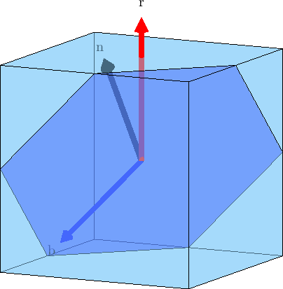

The red arrow is perpendicular to neither the blue arrow nor the black arrow. The loading therefore has a nonzero component that shears this plane along \(\mathbf b\).

Define the Schmid factor

For uniaxial tension, the signed Schmid factor \(m\) is the product of two direction cosines:

\[m = \cos\angle(\mathbf r,\mathbf n)\, \cos\angle(\mathbf r,\mathbf b).\]

A zero factor means that \(\mathbf r\) is perpendicular to either \(\mathbf b\) or \(\mathbf n\). The system then receives no resolved shear. The sign selects the shear sense; activation comparisons usually use \(m\) when opposite Burgers-vector signs are identified.

m = cos(angle(r,sS.n,'noSymmetry')) * ...
  cos(angle(r,sS.b,'noSymmetry'))

m =
   -0.4082

The SchmidFactor method performs the same calculation. Both routes give \(m=-0.4082\) for this signed system.

sS.SchmidFactor(r)

ans =
   -0.4082

Map one system over every tension direction

If the tension direction is omitted, SchmidFactor returns an S2FunHarmonic spherical function. It can be plotted or searched without first constructing a direction grid.

SF = sS.SchmidFactor
plot(SF)

[SFMax,pos] = max(SF)
annotate(pos)

SF = S2FunHarmonic (Nickel)
  bandwidth: 4
  antipodal: true
 
SFMax =
    0.5000
 
pos = Miller (Nickel)
 antipodal: true
        h       k       l
  -1.4387 -3.1996  0.3231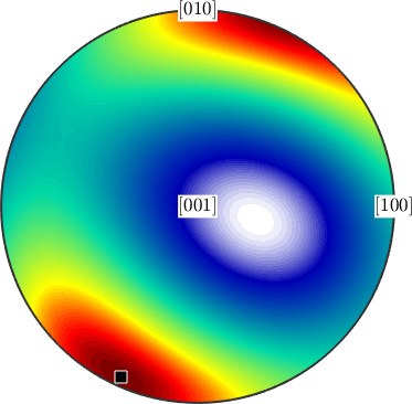

The positive and negative lobes record opposite shear senses. The annotated direction has the theoretical maximum \(m=0.5\): it lies halfway between the slip direction and the plane normal.

Use a general stress tensor

A loading state may instead be supplied as a stressTensor. Here the uniaxial tensor is expressed in the same crystal frame as the system.

sigma = stressTensor.uniaxial(r)
sS.SchmidFactor(sigma)

sigma = stressTensor (Nickel)
  rank: 2 (3 × 3)
 
 *10^-3
     0     0     0
     0     0     0
     0     0 80.57
ans =
   -0.4082

For a stress tensor, SchmidFactor contracts the Schmid tensor with the stress after normalizing by the difference between its largest and smallest principal stresses. The result is dimensionless and lies between \(-0.5\) and \(0.5\). Multiplying by that stress difference gives the resolved shear stress \(\tau\).

Compare all equivalent systems

A crystal contains the symmetry-equivalent systems, not only the chosen representative. The 'antipodal' option identifies opposite Burgers vectors as the two shear senses of the same geometric system.

sSAll = sS.symmetrise('antipodal')

sSAll = slipSystem (Nickel)
 size: 12 × 1
 
   u    v    w  | h    k    l CRSS
   0    1   -1    1    1    1    1
  -1    0    1    1    1    1    1
   1   -1    0    1    1    1    1
   1   -1    0    1    1   -1    1
   1    0    1    1    1   -1    1
   0    1    1    1    1   -1    1
   0    1   -1   -1    1    1    1
   1    0    1   -1    1    1    1
   1    1    0   -1    1    1    1
  -1    0    1    1   -1    1    1
   1    1    0    1   -1    1    1
   0    1    1    1   -1    1    1

The twelve panels show the twelve geometric fcc systems for the fixed red loading direction. Only the plane and Burgers vector change between them.

close all
t = tiledlayout(3,4,'TileSpacing','tight','Padding','tight', ...
  'TileIndexing','columnmajor');
for k = 1:length(sSAll)
  ax = nexttile;
  plot(cS,'faceAlpha',0.5,'parent',ax)
  title(ax,['\textbf{' int2str(k) '}:' char(sSAll(k),'latex')], ...
    'Interpreter','latex')
  axis off
  hold on
  plot(cS,sSAll(k),'facecolor','blue','parent',ax)
  plottingConvention.default3D().setView
  arrow3d(0.4*normalize(r),'faceColor','red','linewidth',3)
  hold off
end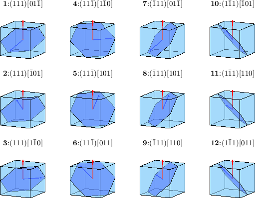

A vectorized call returns one signed factor per system. Taking the largest absolute value finds the system best aligned with this tension axis.

tau = sSAll.SchmidFactor(r)
[tauMax,id] = max(abs(tau))
sSAll(id)

tau =
  Columns 1 through 7
   -0.4082    0.4082    0.0000   -0.0000   -0.4082   -0.4082   -0.4082
  Columns 8 through 12
    0.4082    0.0000    0.4082    0.0000    0.4082
tauMax =
    0.4082
id =
    12
 
ans = slipSystem (Nickel)
 
  u    v    w  | h    k    l CRSS
  0    1    1    1   -1    1    1

The maximum is \(0.4082\) for tension along \([001]\). If systems have different critical resolved shear stresses (CRSS), the option 'relative' divides each factor by its CRSS before the comparison.

tauRelative = sSAll.SchmidFactor(r,'relative');

Map the preferred system

The same vectorized calculation accepts many crystal directions. Rows of tau correspond to directions and columns correspond to slip systems.

rGrid = plotS2Grid('resolution',0.5*degree,'upper',cs.frame);
tau = sSAll.SchmidFactor(rGrid);
[tauMax,id] = max(abs(tau),[],2);

contourf(rGrid,tauMax)
mtexColorbar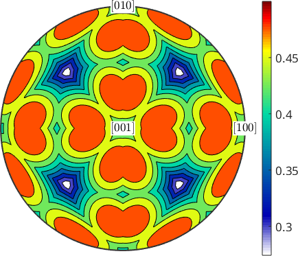

The maximum factor repeats with cubic symmetry. Each curved region is the set of tension directions that selects one member of the slip family.

pcolor(rGrid,id)
mtexColorMap(vega20(12))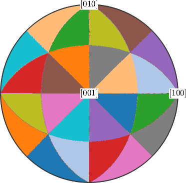

Colour now identifies the selected system rather than the factor itself. The selected index remains constant within each fundamental region. Label the symmetry-related sector centres with their active systems.

rCenter = symmetrise(cs.fundamentalSector.center,cs);
rCenter = rCenter(rCenter.z>=0);
tau = sSAll.SchmidFactor(rCenter);
[~,idCenter] = max(abs(tau),[],2);

hold on
for k = 1:length(rCenter)
  text(rCenter(k),char(sSAll(idCenter(k)),'latex'), ...
    'Interpreter','latex','fontsize',10)
end
hold off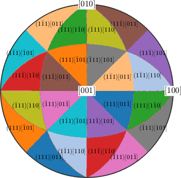

Spherical-function arithmetic gives the same maximum-factor map directly. Omitting r returns one function for each of the twelve systems.

tauFun = sSAll.SchmidFactor
contourf(max(abs(tauFun),[],1),'upper')
mtexColorbar

tauFun = S2FunHarmonic (Nickel)
  size: 12 × 1
  bandwidth: 4
  antipodal: true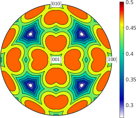

This plot has the same symmetry and extrema as the explicit grid map. Use the grid when the individual direction samples are needed, and use the spherical function for evaluation, plotting, or further arithmetic.

Apply specimen stress to an EBSD map

So far, the stress and slip systems have shared the crystal frame. In an EBSD map, the applied stress is usually expressed in the specimen frame, while each slip system starts in its phase's crystal frame. An orientation maps between those frames.

mtexdata csl

ebsd = ebsd(ebsd.inpolygon([0,0,200,50]));
grains = calcGrains(ebsd);
grains = smoothBoundary(grains,5);

plot(ebsd,ebsd.orientations,'micronbar','off')
hold on
plot(grains.boundary,'linewidth',2)
hold off

ebsd = EBSD (y↓→x)
 
 Phase   Orientations     Mineral         Color  Symmetry  Crystal reference frame
     0    5 (0.0032%)  notIndexed          none                                   
    -1  154107 (100%)        iron  LightSkyBlue      m-3m                         
 
 Properties: ci, error, iq
 Scan unit : um
 X × Y × Z : [0 → 511] × [0 → 300] × [0 → 0]
 Normal vector: (0,0,1)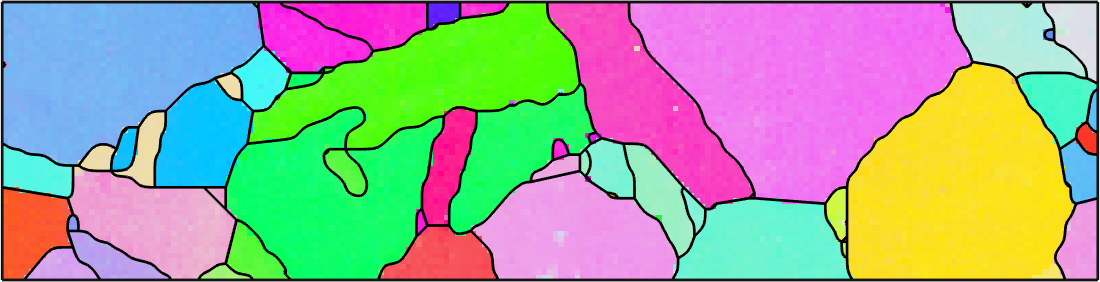

The black outlines delimit grains. Each grain has one mean orientation, which is the frame map used for its Schmid-factor calculation.

sS = slipSystem.fcc(ebsd.CS);
sS = sS.symmetrise;

Rotate the systems into the specimen frame

Calling symmetrise without 'antipodal' retains both Burgers-vector signs. The following product makes one row per grain and one column per symmetrically equivalent slip system, all expressed in the specimen frame.

sSLocal = grains.meanOrientation * sS;

sigma = stressTensor.uniaxial(vector3d.Z)
SFSpecimen = sSLocal.SchmidFactor(sigma);
[SFMax,active] = max(SFSpecimen,[],2);

plot(grains,SFMax,'micronbar','off','linewidth',2)
mtexColorbar southoutside

sigma = stressTensor (y↓→x)
  rank: 2 (3 × 3)
 
 0 0 0
 0 0 0
 0 0 1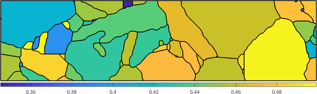

Bright grains have a slip system well aligned with specimen \(z\) tension. Dark grains require more applied stress to reach the same CRSS.

sSActive = grains.meanOrientation .* sS(active);

hold on
quiver(grains,sSActive.trace,'color','b')
quiver(grains,sSActive.b,'color','r')
hold off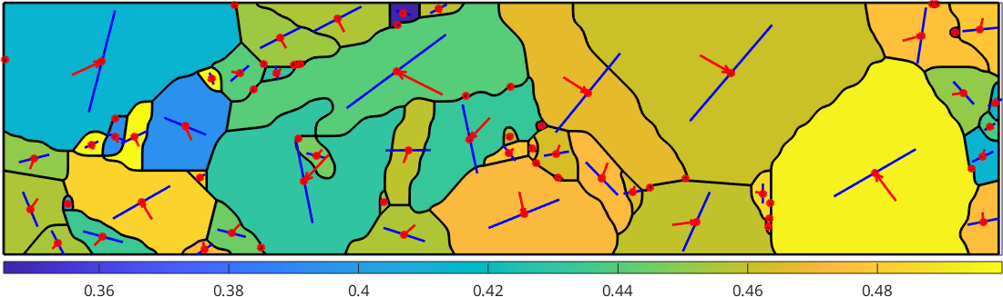

Blue arrows show the surface traces of the active slip planes, and red arrows show the Burgers vectors. They align when the Burgers vector lies in the map surface. A mismatch shows that the slip direction has a component out of the surface.

Alternatively, rotate the stress into each crystal frame

The equivalent route leaves the systems in their crystal frame and maps the specimen stress back with the inverse grain orientations.

sigmaLocal = inv(grains.meanOrientation) * sigma;
SFCrystal = sS.SchmidFactor(sigmaLocal);

Both inputs now share a crystal frame. The two routes agree to numerical roundoff, so either may be chosen according to the next calculation.

max(abs(SFCrystal-SFSpecimen),[],'all')

[SFMax,active] = max(SFCrystal,[],2);
plot(grains,SFMax,'micronbar','off','linewidth',2)
mtexColorbar southoutside

sSActive = grains.meanOrientation .* sS(active);
hold on
quiver(grains,sSActive.trace,'color','b')
quiver(grains,sSActive.b,'color','r')
hold off

ans =
   3.1919e-16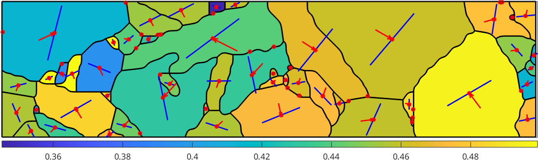

This final map and its arrows reproduce the specimen-frame result. A frame mismatch instead triggers an MTEX:frameMismatch warning, because the resulting factors would have no physical meaning.

References

Next

Schmid analysis selects systems under an imposed stress. Continue with Taylor Model to find the combination of slip systems that accommodates an imposed strain.

References

- U. F. Kocks, C. N. Tomé and H.-R. Wenk, Texture and Anisotropy, Cambridge University Press, 1998, derives Schmid's law and relates resolved shear stress to slip-system activation.