Basic Settings
display pole figure plots with RD on top and ND west
plotzOutOfPlane, plotx2north

% store old annotation style
storepfA = getMTEXpref('pfAnnotations');

% set new annotation style to display RD and ND
pfAnnotations = @(varargin) text(-[vector3d.X,vector3d.Y],{'RD','ND'},...
  'BackgroundColor','w','tag','axesLabels',varargin{:});

setMTEXpref('pfAnnotations',pfAnnotations);
Slip in Body Centered Cubic Materials
In the following we consider crystallographic slip in bcc materials
% define the slip systems in bcc
cs = crystalSymmetry('432');
sS = slipSystem.bcc(cs)
sS = slipSystem (432)
size: 1 x 3
u v w | h k l CRSS
1 -1 1 0 1 1 1
-1 1 1 2 1 1 1
-1 1 1 3 2 1 1under plane strain
q = 0;
epsilon = strainTensor(diag([1 -q -(1-q)]))
epsilon = strainTensor (y↑→x)
type: Lagrange
rank: 2 (3 x 3)
1 0 0
0 0 0
0 0 -1The orientation dependence of the Taylor factor
For a family of slip systems sS the Taylor factor M describes the total amount of slip activity that is required to deform a crystal in orientation ori according to strain epsilon. In MTEX this can be computed by the command calcTaylor.
% define a crystal orientation
ori = orientation.byEuler(0,30*degree,15*degree,cs)

% compute the Taylor factor
[M,b,W] = calcTaylor(inv(ori)*epsilon,sS.symmetrise);

M
W
ori = orientation (432 → y↑→x)
Bunge Euler angles in degree
phi1 Phi phi2
0 30 15
M =
2.1208
W = spinTensor (432)
rank: 2 (3 x 3)
*10^-2
0 51 65.65
-51 0 -23.04
-65.65 23.04 0When called without specifying an orientation the command calcTaylor computes the Taylor factor M as well as the spin tensors W as orientation dependent functions, which can be easily visualized and analyzed.
[M,~,W] = calcTaylor(epsilon,sS.symmetrise)

% evaluate the Taylor factor at an arbitrary orientation
M.eval(ori)
W.eval(ori)
M = SO3FunHarmonic (432 → y↑→x)
bandwidth: 32
weight: 3.1
W = SO3VectorFieldHarmonic (1 → y↑→x)
bandwidth: 32
tangent space: rightSpinTensor
intern symmetries: 432 → y↑→x
intern tangent space: leftVector
ans =
2.1009
ans = spinTensor (y↑→x)
rank: 2 (3 x 3)
*10^-2
0 38.89 49.68
-38.89 0 -14.97
-49.68 14.97 0The following code reproduces Fig. 5 of the paper of Bunge, H. J. (1970). Some applications of the Taylor theory of polycrystal plasticity. Kristall Und Technik, 5(1), 145-175. http://doi.org/10.1002/crat.19700050112
% set up an phi1 section plot
sP = phi1Sections(cs);
sP.phi1 = (0:10:90)*degree;

% plot the Taylor factor
plot(M,'smooth',sP)
mtexColorbar

hold on
plot(W,'color','black')
hold off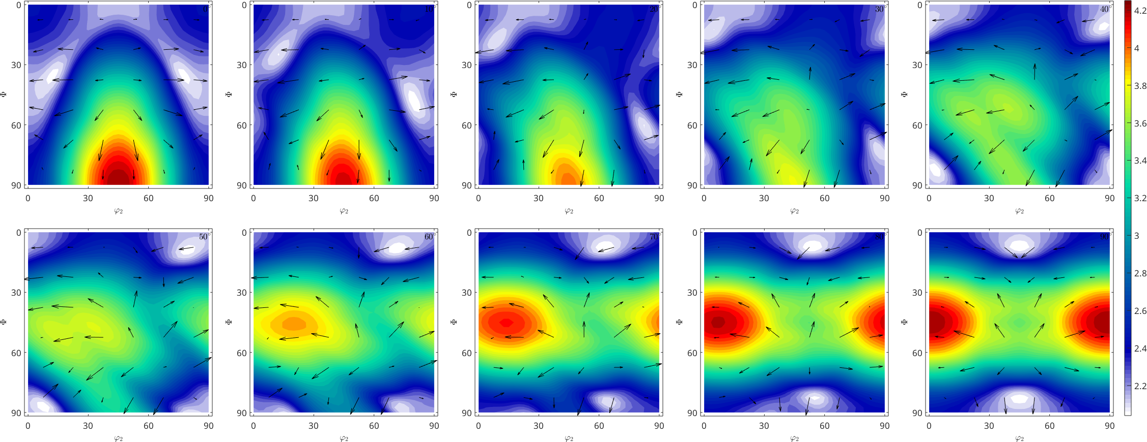
The orientation dependence of the spin
The norm of the spin tensor is exactly the angle of misorientation a crystal with the corresponding orientation experiences according to Taylor theory. Compare Fig. 8 of the above paper
plot(norm(W)/degree,'smooth',sP,'resolution',0.5*degree)
mtexColorbar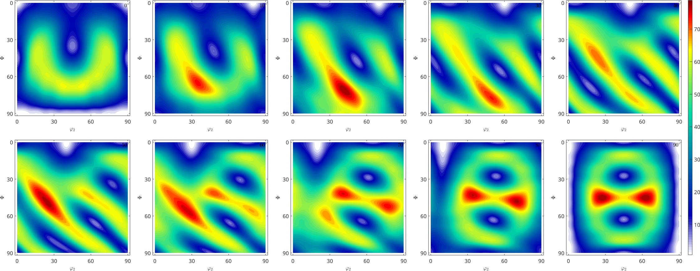
Display the crystallographic spin in sigma sections
sP = sigmaSections(cs);
plot(norm(W)./degree,'smooth',sP)
mtexColorbar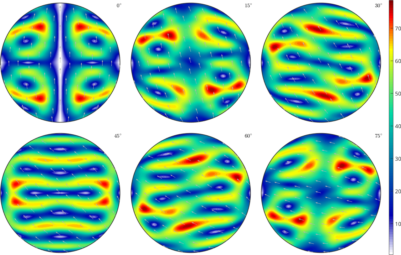
Identification of the most active slip directions
Next we consider a real world data set
mtexdata csl

% compute grains
grains = calcGrains(ebsd('indexed'),'minPixel',3);
grains = smooth(grains,5);
ebsd = EBSD (y↑→x)
Phase Orientations Mineral Color Symmetry Crystal reference frame
0 5 (0.0032%) notIndexed
-1 154107 (100%) iron LightSkyBlue m-3m
Properties: ci, error, iq
Scan unit : um
X x Y x Z : [0, 511] x [0, 300] x [0, 0]
Normal vector: (0,0,1)and apply the Taylor model to each grain of our data set
% some strain
q = 0;
epsilon = strainTensor(diag([1 -q -(1-q)]))

% consider fcc slip systems
sS = symmetrise(slipSystem.fcc(grains.CS));

% apply Taylor model
[M,b,W] = calcTaylor(inv(grains.meanOrientation)*epsilon,sS);
epsilon = strainTensor (y↑→x)
type: Lagrange
rank: 2 (3 x 3)
1 0 0
0 0 0
0 0 -1% colorize grains according to Taylor factor
plot(grains,M)
mtexColorMap white2black
mtexColorbar
% index of the most active slip system - largest b
[~,bMaxId] = max(b,[],2);
% rotate the most active slip system in specimen coordinates
sSGrains = grains.meanOrientation .* sS(bMaxId);
% visualize slip direction and slip plane for each grain
hold on
quiver(grains,sSGrains.b,'autoScaleFactor',0.7,'displayName','Burgers vector','project2plane')
hold on
quiver(grains,sSGrains.trace,'autoScaleFactor',0.7,'displayName','slip plane trace')
hold off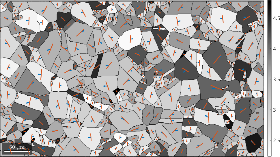
plot the most active slip directions observe that they point all towards the lower hemisphere - why? they do change if q is changed
figure(2)
plot(sSGrains.b)
text([xvector,yvector,zvector],'labeled','BackGroundcolor','w')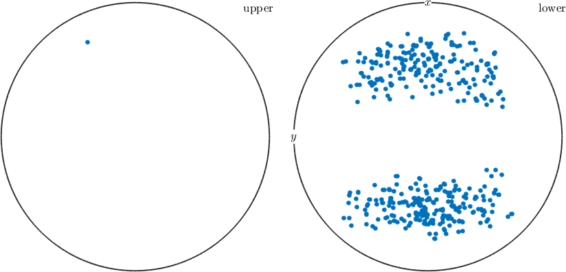
Texture evolution during rolling
% define some random orientations
rng(0)
ori = orientation.rand(1e5,grains.CS);

% 30 percent plane strain
q = 0;
epsilon = 0.3 * strainTensor(diag([1 -q -(1-q)]));

numIter = 100;

% compute the Taylor factors and the orientation gradients
[~,~,spin] = calcTaylor(epsilon ./ numIter, sS.symmetrise);

pC = progressCounter(numIter);
for sas = 1:numIter

  % compute the Taylor factors and the orientation gradients
  W = spinTensor(spin.eval(ori).').';

  % rotate the individual orientations
  ori = ori .* orientation(-W);
  pC.show(sas);

end
% plot the resulting pole figures
% set new annotation style to display RD and ND
pfAnnotations = @(varargin) text([vector3d.X,vector3d.Y,vector3d.Z],{'RD','TD','ND'},...
'BackgroundColor','w','tag','axesLabels',varargin{:});
setMTEXpref('pfAnnotations',pfAnnotations);
plotPDF(ori,Miller({0,0,1},{1,1,1},cs),'contourf')
mtexColorbar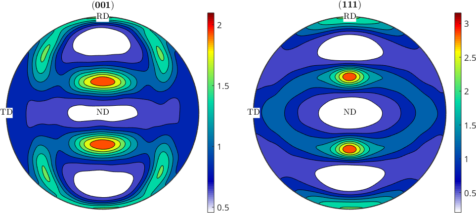
restore MTEX preferences
close all
setMTEXpref('pfAnnotations',storepfA);