Orientation maps determined by EBSD or any other technique are, as all experimental data, effected by measurement errors. Those measurement errors can be divided into systematic errors and random errors. Systematic errors mostly occur due to a bad calibration of the EBSD system and require additional knowledge to be corrected. Deviations from the true orientation due to noisy Kikuchi pattern or tolerances of the indexing algorithm can be modeled as random errors. In this section we demonstrate how random errors can be significantly reduced using denoising techniques.
Denoising orientation maps may also include filling not indexed pixels. This is explained in the section Fill Missing Data.
We shall demonstrate the denoising capabilities of MTEX at the hand of an orientation map of deformed Magnesium.
% import the data
mtexdata twins

% reconstruct the grain structure
[grains,ebsd.grainId] = calcGrains(ebsd('indexed'),'angle',10*degree,'minPixel',5);

% smooth grain boundaries
grains = smooth(grains,5);

% consider only indexed data
ebsd = ebsd('indexed');

% plot the orientation map
ipfKey = ipfColorKey(ebsd.CS.properGroup);
plot(ebsd,ipfKey.orientation2color(ebsd.orientations))

% and on top the grain boundaries
hold on
plot(grains.boundary,'linewidth',2,'linecolor','white')
hold off
ebsd = EBSD (y↑→x)
Phase Orientations Mineral Color Symmetry Crystal reference frame
0 46 (0.2%) notIndexed
1 22833 (100%) Magnesium LightSkyBlue 6/mmm X||a*, Y||b, Z||c*
Properties: bands, bc, bs, error, mad
Scan unit : um
X x Y x Z : [0, 50] x [0, 41] x [0, 0]
Normal vector: (0,0,1)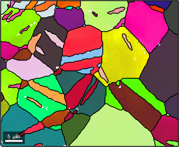
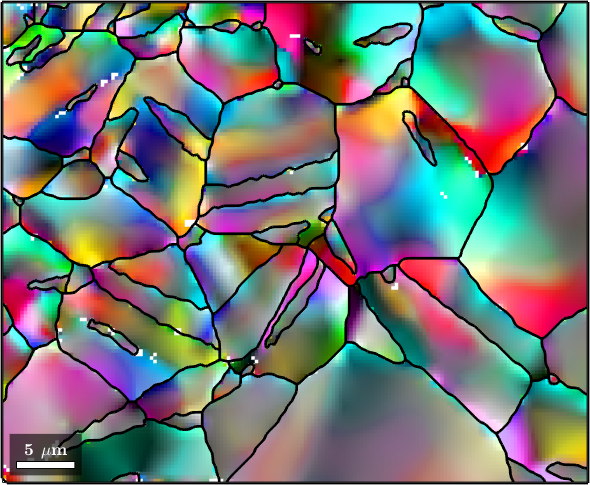
At the first glance, the orientation data look not noisy at all. However, if we look at orientation changes within the grains the noise becomes clearly visible. To do so we colorize the orientation data with respect to their misorientation to the grain mean orientation
% the axisAngleColorKey colorizes misorientation according to their axis and angle
colorKey = axisAngleColorKey;

% we set the reference orientations as the mean orientation of each grain
colorKey.oriRef = grains(ebsd.grainId).meanOrientation;

% lets plot the result
plot(ebsd,colorKey.orientation2color(ebsd.orientations))
hold on
plot(grains.boundary,'linewidth',2)
hold off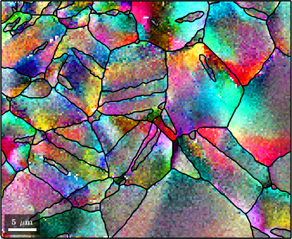
We clearly observe some deformation gradients withing the grains which are superposed by random noise. In the following we discuss several methods for noise removal. The by far best method is the total variation filter discussed further down the list.
The Mean Filter
The simplest filter to apply to orientation data is the meanFilter which replaces all orientations by the mean of all neighboring orientations.
% define the meanFilter
F = meanFilter;
F.numNeighbours = 1;

% smooth the data
ebsdS = smooth(ebsd,F);
ebsdS = ebsdS('indexed');

% plot the smoothed data
colorKey.oriRef = grains(ebsdS.grainId).meanOrientation;
plot(ebsdS, colorKey.orientation2color(ebsdS.orientations))

hold on
plot(grains.boundary,'linewidth',2)
hold off
We clearly see how the noise has been reduces. In order to further reduce the noise we may increase the number of neighbors that are taken into account.
F.numNeighbours = 3;

% smooth the data
ebsdS = smooth(ebsd,F);
ebsdS = ebsdS('indexed');

% plot the smoothed data
colorKey.oriRef = grains(ebsdS.grainId).meanOrientation;
plot(ebsdS,colorKey.orientation2color(ebsdS.orientations))

hold on
plot(grains.boundary,'linewidth',2)
hold off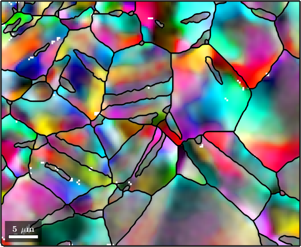
The Median Filter
The disadvantage of the mean filter is that is smoothes away all subgrain boundaries and is quite sensitive against outliers. A more robust filter which also preserves subgrain boundaries is the median filter
F = medianFilter;

% define the size of the window to be used for finding the median
F.numNeighbours = 3; % this corresponds to a 7x7 window

% smooth the data
ebsdS = smooth(ebsd,F);
ebsdS = ebsdS('indexed');

% plot the smoothed data
colorKey.oriRef = grains(ebsdS.grainId).meanOrientation;
plot(ebsdS,colorKey.orientation2color(ebsdS.orientations))

hold on
plot(grains.boundary,'linewidth',2)
hold off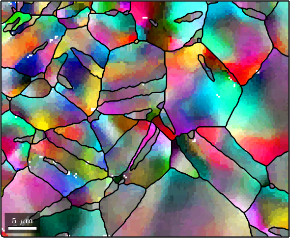
The disadvantage of the median filter is that it leads to cartoon like images which suffer from the staircase effect.
The Kuwahara Filter
Another filter that was designed to be robust against outliers and does not smooth away subgrain boundaries is the Kuwahara filter. However, in practical applications the results are often not satisfactory.
F = KuwaharaFilter;
F.numNeighbours = 5;

% smooth the data
ebsdS = smooth(ebsd,F);
ebsdS = ebsdS('indexed');

% plot the smoothed data
colorKey.oriRef = grains(ebsdS.grainId).meanOrientation;
plot(ebsdS,colorKey.orientation2color(ebsdS.orientations))

hold on
plot(grains.boundary,'linewidth',2)
hold off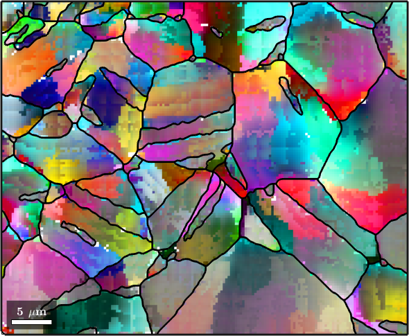
The Smoothing Spline Filter
All the above filters are so called sliding windows filters which consider for the denoising operation only neighboring orientations within a certain window. The next filters belong to the class of variational filters which determine the denoised orientation map as the solution of an minimization problem that is simultaneously close to the original map and "smooth". The resulting orientation map heavily depends on the specific definition of "smooth" and on the regularization parameter which controls the trade of between fitting the original data and forcing the resulting map to be smooth.
The splineFilter uses as definition of smoothness the curvature of the orientation map. As a consequence, the denoised images are very "round" and similarly as for the meanFilter subgrain boundaries will be smoothed away. On the positive side the meanFilter is up to now the only filter that automatically calibrates the regularization parameter.
F = splineFilter;

% smooth the data
ebsdS = smooth(ebsd,F);
ebsdS = ebsdS('indexed');

% plot the smoothed data
colorKey.oriRef = grains(ebsdS.grainId).meanOrientation;
plot(ebsdS,colorKey.orientation2color(ebsdS.orientations))

hold on
plot(grains.boundary,'linewidth',2)
hold off

% the smoothing parameter determined during smoothing is
F.alpha
ans =
4.6123
The Total Variation Filter
In the default setting the halfQuadraticFilter uses definition of smoothness the total variation functional. This functional was developed to preserve subgrain boundaries. Similarly as the medianFilter it tends to carton like images and staircasing.
F = halfQuadraticFilter;

% smooth the data
ebsdS = smooth(ebsd,F);
ebsdS = ebsdS('indexed');

% plot the smoothed data
colorKey.oriRef = grains(ebsdS.grainId).meanOrientation;
plot(ebsdS,colorKey.orientation2color(ebsdS.orientations))

hold on
plot(grains.boundary,'linewidth',2)
hold off
The Infimal Convolution Filter
The infimal convolution filter was designed as a compromise between the splineFilter and the halfQuadraticFilter. It is still under development and its use is not recommended.
F = infimalConvolutionFilter;
F.lambda = 0.01; % smoothing parameter for the gradient
F.mu = 0.005;    % smoothing parameter for the hessian

% smooth the data
ebsdS = smooth(ebsd,F);
ebsdS = ebsdS('indexed');

% plot the smoothed data
colorKey.oriRef = grains(ebsdS.grainId).meanOrientation;
plot(ebsdS,colorKey.orientation2color(ebsdS.orientations))

hold on
plot(grains.boundary,'linewidth',2)
hold off