Fibre ODFs

A fibre ODF is a density concentrated around a one-dimensional orientation fibre. Every orientation on it maps one fixed crystal direction onto one fixed specimen direction. Rotation about that aligned direction remains free, so the ODF is constant along the fibre and decays across it.

Wire drawing gives the classical example. A crystal direction from the \(\langle111\rangle\) family aligns with the drawing axis. Rotation about that axis remains unconstrained. The ideal fibre has zero width. A fibre ODF replaces it by a normalized tube of finite angular width.

This page assumes the ODF normalization introduced in ODF Theory. ODF Modeling introduces the model families. The geometry and named rolling-texture fibres are developed in Fibres of Orientations.

The plotting convention below draws specimen Y upward and specimen X to the right. It changes only the screen layout, not the ODF or its reference frames.

plottingConvention.default('y↑→x');

Defining a Fibre ODF

A fibre is represented by an object of type fibre. Many of the named fibres of rolling textures are built in. This example uses the built-in beta fibre for a cubic rolling texture. Its printed summary gives the endpoint orientations. It also gives the crystal and specimen directions that remain parallel.

cs = crystalSymmetry('432');
f = fibre.beta(cs)

f = fibre (432 → y↑→x)
 
  h || r: (12 6 11) || (-1,-1,4)
 o1 → o2: (180°,35.3°,45°) → (270°,62.8°,45°)

The displayed h parallel r row puts the two directions in different reference frames: f.h belongs to the crystal frame and f.r to the specimen frame. The beta object also has two endpoints. fibreODF uses only the direction pair, so the density continues around the corresponding full fibre.

The 'halfwidth' option controls how quickly the density decays away from that fibre. The returned summary identifies the SO3FunCBF representation, its kernel, halfwidth, defining directions, and weight.

odf = fibreODF(f,'halfwidth',10*degree)

odf = SO3FunCBF (432 → y↑→x)
 
  kernel: de la Vallee Poussin, halfwidth 10°
  fibre : (12 6 11) || -1,-1,4
  weight: 1

The Tube in Orientation Space

A three-dimensional contour plot shows surfaces of equal density around the fibre.

plot3d(odf);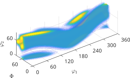

The translucent branches are sections of one tubular ridge folded by cubic symmetry. They are symmetry-equivalent descriptions of the same fibre component, not additional physical components.

Sections Through the Tube

A sigma-section plot cuts through the same tube. The ridge passes from panel to panel because a section shows only a slice of the three-dimensional orientation space.

plotSection(odf,'sigma');
mtexColorbar('title','mrd');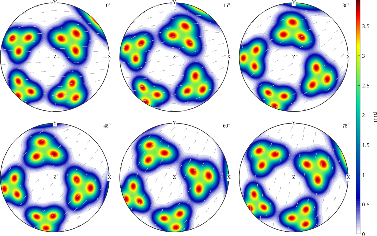

The brightest curves trace the fibre through the section panels. Their intensity stays constant along the centreline. The surrounding colour bands show the decay across it. Evaluate 25 orientations on the original beta segment to check that constancy directly.

oriOnFibre = orientation(f,'points',25);
ridgeValueRange = [min(eval(odf,oriOnFibre)),max(eval(odf,oriOnFibre))]

ridgeValueRange =
    3.9239    3.9239

Pole Figures of a Fibre ODF

A pole figure projects an ODF by integrating along orientation fibres. Plot the defining crystal direction first, followed by the standard \((100)\) and \((111)\) directions. Pole Figures of an ODF develops this projection as the crystallographic Radon transform.

h = [f.h,Miller(1,0,0,cs),Miller(1,1,1,cs)];
plotPDF(odf,h,'contourf');
mtexColorbar('title','mrd');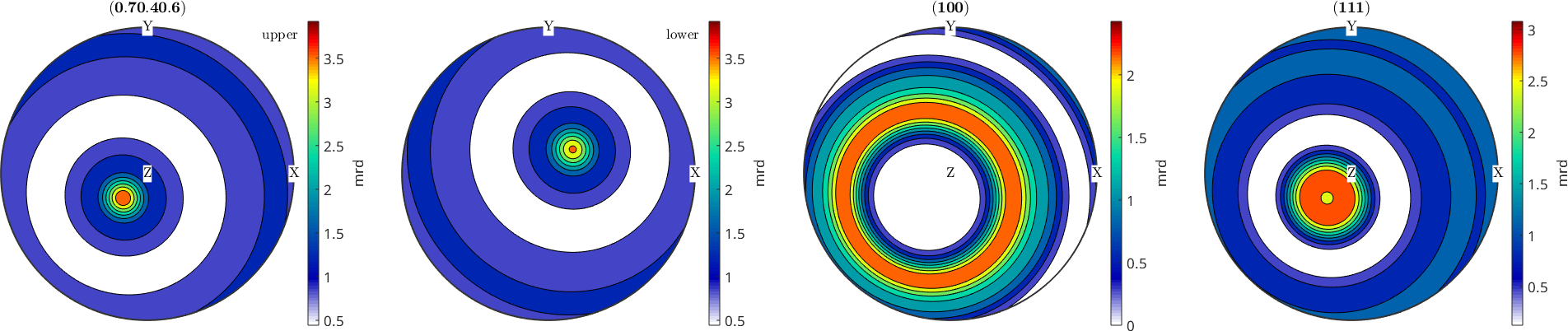

For the ideal fibre, its defining direction collapses to the specimen direction f.r and its symmetry-equivalent copies. The finite halfwidth broadens each point into a spot in the first panel. The other directions sweep rings or ring segments about f.r. A ring is therefore a projection of the fibre, not a second component.

The Effect of the Halfwidth

This example uses the default de la Vallee Poussin kernel. Its halfwidth is the angular distance at which density falls to half its ridge value. It is a spread parameter, not a cutoff: the density continues beyond that angle. fibreODF also accepts a custom S2Kernel when halfwidth alone does not describe the required shape. ODF Shapes compares the kernels.

Each component below remains normalized with mean 1 mrd. Narrower fibres concentrate that same total volume into a smaller tube, so their maximum and texture index are larger. Neither number is a volume fraction.

halfwidths = [5 10 20]*degree;
odfByHalfwidth = cell(size(halfwidths));
for i = 1:numel(halfwidths)
  odfByHalfwidth{i} = fibreODF(f,'halfwidth',halfwidths(i));
  fprintf(['halfwidth %4.1f degree : mean %4.2f, texture index %6.2f, ' ...
    'maximum %6.2f\n'],halfwidths(i)./degree,mean(odfByHalfwidth{i}),...
    norm(odfByHalfwidth{i})^2,max(odfByHalfwidth{i}));
end

halfwidth  5.0 degree : mean 1.00, texture index   7.62, maximum  15.21
halfwidth 10.0 degree : mean 1.00, texture index   2.36, maximum   3.93
halfwidth 20.0 degree : mean 1.00, texture index   1.26, maximum   2.06

The pole density around the defining specimen direction broadens as the halfwidth increases. A shared colour range also makes the fall in peak density visible from left to right.

mtexFig = newMtexFigure('layout',[1,3],'figSize','large');
for i = 1:numel(halfwidths)
  plotPDF(odfByHalfwidth{i},f.h,'contourf','noTitle');
  mtexTitle(['\(' xnum2str(halfwidths(i)./degree) '^{\circ}\)']);
  if i < numel(halfwidths), nextAxis; end
end
setColorRange('equal');
mtexColorbar('title','mrd');
drawNow(mtexFig);

Fitting a Fibre to Data

The inverse problem asks which fibre best describes an ODF or a set of orientations. fibre.fit returns a candidate centreline. Start with a low-symmetry fibre so that every sampled orientation has one consistent representative. The 'local' branch then reads the fibre from the orientation tensor without a global grid search. The sampling step is developed separately in Random Sampling.

csFit = crystalSymmetry('1');
fTrue = fibre(Miller(1,1,1,csFit),vector3d.Z);
odfFit = fibreODF(fTrue,'halfwidth',10*degree);
ori = discreteSample(odfFit,1000);
[fFit,lambda,fitDistance] = fibre.fit(ori,'local');
fFit

fFit = fibre (1 → y↑→x)
 
  h || r: (1̅1̅1̅) || (0,0,-1)
 o1 → o2: (193.7°,54.5°,45.2°) → (193.7°,54.5°,45.2°)

The two printed distances are the sample's mean angular distance from the true fibre and from the fitted fibre. They should be similar for this synthetic low-symmetry example.

meanDistanceDegrees = ...
  [mean(angle(ori,fTrue)),fitDistance] ./ degree

meanDistanceDegrees =
    7.5823    7.5661

The eigenvalues returned by the local branch test whether a fibre is a sensible model. The ratio below compares spread along the fibre with scatter away from it. A ratio near 1 describes a blob rather than a line; a larger ratio supports a fibre interpretation.

linearityRatio = lambda(3)./lambda(2)

linearityRatio =
  161.2818

Two warnings are essential. First, the fit always returns a fibre even when the data do not follow one. Applied to a unimodal ODF, it can simply return a fibre through the mode. Dispersion Axes develops the eigenvalue diagnostic with measured grain orientations.

Second, the global search is not reliable for highly symmetric groups. On cubic data, compare the mean distance to the fitted fibre with the distance to any physically expected fibre. A larger fitted distance is the clear failure symptom seen in the original cubic example. Treat a cubic global fit as a starting point for manual inspection.

The local branch is much faster, but it requires low symmetry. It can also use a good starting guess that has already put symmetry-equivalent observations into one locally consistent set. The API does not accept the starting guess itself.

The Maths Behind a Fibre ODF

For a crystal direction \(h\) and a specimen direction \(r\), the full fibre is

\[F_{h,r}=\{g \in SO(3):g h=r\}.\]

Away from symmetry equivalents, a single fibre component has the form

\[f(g)=\psi(\angle(g h,r)),\]

where \(\psi\) is the spherical kernel. Crystal and specimen symmetry make the construction invariant under equivalent descriptions. MTEX stores the object as an SO3FunCBF. It still uses the evaluation, plotting, scaling, and addition interface shared by every SO3Fun.

Further Reading

Next

Continue with Bingham ODFs for a compact parametric model with three independent spreads. The preceding model family is Radial ODFs, and the curves without a density around them are Fibres of Orientations. ODF Properties explains texture index and fibre volume. Density Estimation estimates an ODF from measured orientations instead of fitting a single parametric centreline.