Slip Transmission

Slip that reaches a grain boundary may continue on a suitably aligned system in the neighbouring grain. Slip transmission is this transfer of plastic shear across the boundary. It depends on the systems selected on both sides, so it connects the independent-grain models from the preceding pages to an observable grain-to-grain interaction.

This page selects basal slip under uniaxial tension, maps the Luster--Morris \(m'\) compatibility parameter on every boundary segment, and then shows how compatibility varies with misorientation.

Reconstruct the titanium grains

Load the alpha-titanium EBSD map contributed by D. Mercier for the 2016 MTEX workshop in Chemnitz. A grain is a phase-homogeneous, spatially connected region of EBSD pixels produced by segmentation.

mtexdata titanium

[grains,ebsd] = calcGrains(ebsd);
grains = smoothBoundary(grains);

ebsd = EBSDhex (y↓→x)
 
 Phase  Orientations           Mineral         Color  Symmetry  Crystal reference frame
     0    8100 (99%)  Titanium (Alpha)  LightSkyBlue       622        X||a, Y||b*, Z||c
 
 Properties: ci, grainid, iq, sem_signal, oldId
 Scan unit : um
 X × Y × Z : [0 → 996] × [0 → 998] × [0 → 0]
 Normal vector: (0,0,1)
 Hex grid     :97 × 84

Retain boundary segments whose two neighbouring grains are indexed. These are the segments for which both mean orientations define slip systems.

gB = grains.boundary('indexed');

plot(ebsd,ebsd.orientations)
hold on
plot(grains.boundary)
hold off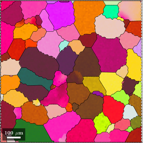

The coloured pixels show crystal orientation, and the black lines delimit the reconstructed grains. Transmission will be evaluated only along the internal indexed boundaries collected in gB.

Select a basal system in every grain

Alpha titanium has three geometric basal systems. Here symmetrise retains both shear senses, giving six signed candidates per grain.

sSBasal = slipSystem.basal(ebsd.CS)
sSBasal = sSBasal.symmetrise;

sSBasal = slipSystem (Titanium (Alpha))
 
  U    V    T    W  | H    K    I    L CRSS
  1    1   -2    0    0    0    0    1    1

Apply uniaxial tension along specimen \(x\). The inverse mean orientation maps that direction into the crystal frame of every grain. The resulting matrix has one row per grain and one column per signed basal system.

SFDirection = sSBasal.SchmidFactor( ...
  inv(grains.meanOrientation) * xvector);

[SFMax,idActive] = max(SFDirection,[],2);

plot(grains,SFMax)
mtexColorbar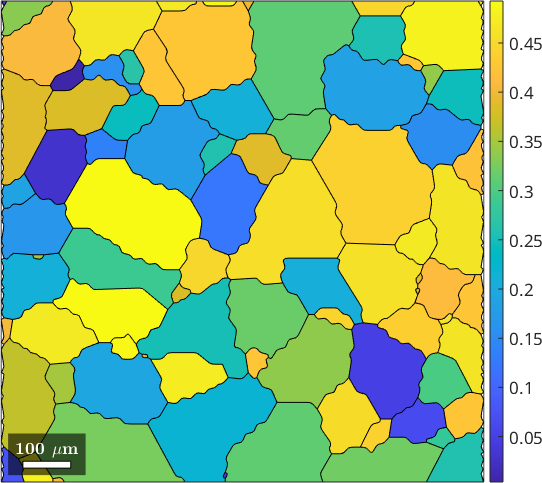

Bright grains have a basal system close to the optimum Schmid factor of 0.5. Dark grains are poorly oriented for basal slip under this load. The vector idActive identifies the selected signed system in every grain.

Draw the selected systems in the specimen frame

Rotate each selected system from its crystal frame into the specimen frame. The blue arrow is the surface trace of the slip plane, and the red arrow is the projected Burgers vector.

sSGrain = grains.meanOrientation .* sSBasal(idActive)

hold on
quiver(grains,sSGrain.trace,'displayName','slip plane')
quiver(grains,sSGrain.b,'displayName','slip direction', ...
  'project2plane')
hold off
legend Location northeast

sSGrain = slipSystem (y↓→x)
 CRSS: 1
 size: 85 × 1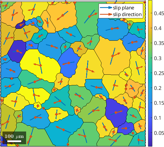

Neighbouring grains often select visibly different plane traces and slip directions. The boundary calculation below measures how well each such pair aligns in three dimensions, not merely in this map projection.

Inspect the selected slip directions

A pole figure retains every selected Burgers vector as one point.

plot(sSGrain.b)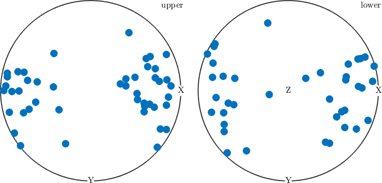

The point cloud is not uniform. More selected directions lie near the east--west axis than near the north--south axis.

plot(sSGrain.b,'contourf')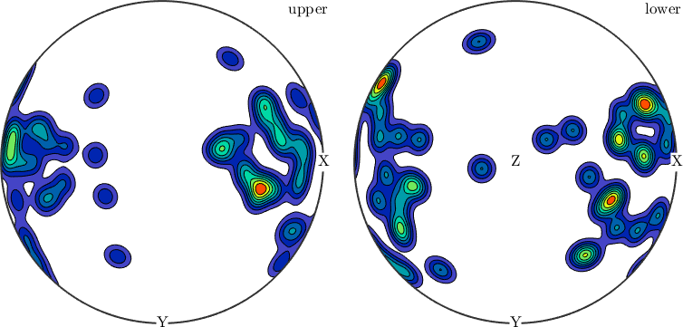

The contour plot summarizes the same points as a density. Its east--west maximum makes the preferred trend easier to see, while the point plot preserves the individual grain predictions.

Use an equivalent stress tensor

A stressTensor is required for a loading state that cannot be represented by one tension direction. For the same uniaxial \(x\) tension, however, the direction and tensor routes should agree.

sigma = stressTensor.uniaxial(xvector);
SFStress = sSBasal.SchmidFactor( ...
  inv(grains.meanOrientation) * sigma);
[SFMaxStress,idStress] = max(SFStress,[],2);

max(abs(SFMaxStress-SFMax))
nnz(idStress~=idActive)

ans =
   3.3307e-16
ans =
     0

The maximum difference is \(3.33\times10^{-16}\), which is numerical roundoff, and zero grains change system. Although an earlier version of this page said that the result was "a bit different," it is not different for the same uniaxial load. A genuinely multiaxial stress can select a different system and must use the tensor route.

Map compatibility on the boundaries

The Luster--Morris parameter \(m'\) compares the slip-plane normals and slip directions on opposite sides of a boundary. A value near one means both pairs are nearly parallel. A value near zero means that at least one pair is nearly perpendicular.

boundaryGrainIds = gB.grainId;
mPBoundary = mPrime( ...
  sSGrain(boundaryGrainIds(:,1)), ...
  sSGrain(boundaryGrainIds(:,2)));

plot(grains,'FaceColor',0.8*[1 1 1],'figSize','large')
hold on
plot(gB,mPBoundary,'linewidth',3)
mtexColorbar
quiver(grains,sSGrain.trace,'displayName','slip plane')
quiver(grains,sSGrain.b,'displayName','slip direction', ...
  'project2plane')
hold off
legend Location northeast

mPStats = [min(mPBoundary),median(mPBoundary),max(mPBoundary)]

mPStats =
    0.0001    0.3719    0.9611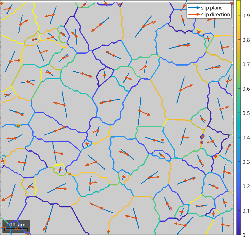

Bright boundary segments connect selected systems with high geometric compatibility; dark segments connect poorly aligned systems. The minimum, median, and maximum are 0.00007, 0.37, and 0.96. The wide range shows why grain orientation alone does not imply uniform transmission through the map.

Plot the best compatibility in misorientation space

The \(m'\) value is unchanged if both crystals and both systems are rotated together. It therefore depends on their relative misorientation. An axis--angle section plot can show this dependence without referring to a particular EBSD map.

sP = axisAngleSections(sSBasal.CS,sSBasal.CS);
moriGrid = sP.makeGrid;

Fix one incoming basal system. At each misorientation, compare it with all symmetry-equivalent outgoing basal systems and retain the best \(m'\).

sSBasalReference = slipSystem.basal(ebsd.CS);
mPGrid = max(mPrime(sSBasalReference, ...
  moriGrid * sSBasalReference.symmetrise),[],2);

sP.plot(mPGrid,'smooth')
mtexColorbar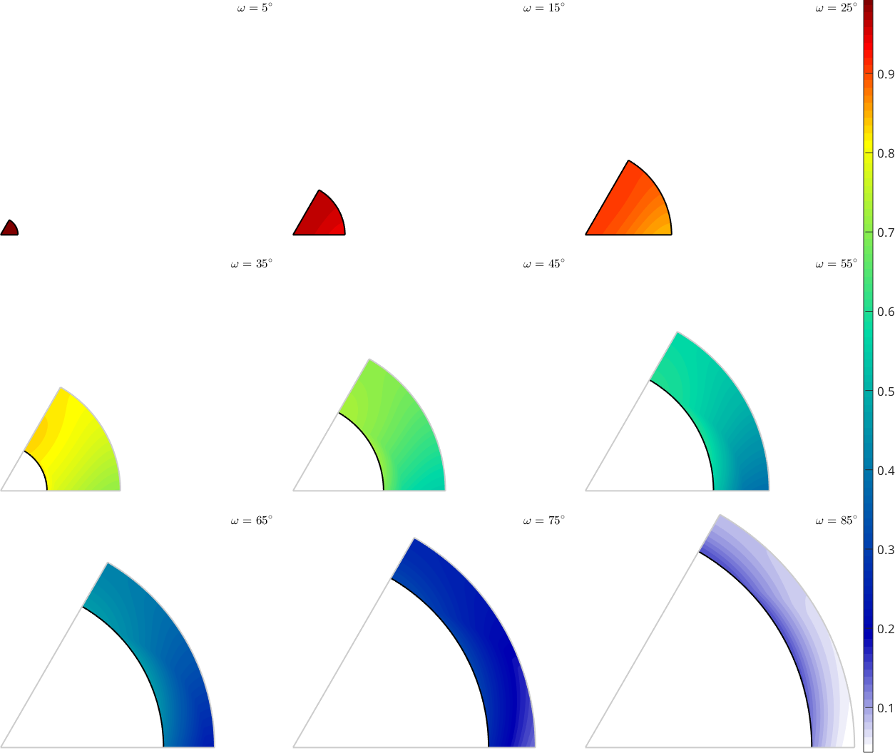

The colour map runs from white at the bottom of the range through blue, green and yellow to dark red at the top. The dark red regions are the misorientations for which at least one outgoing basal system nearly continues the incoming one. The white regions offer no similarly aligned basal system. Unlike the boundary map, this plot chooses the best outgoing system without considering the applied stress.

What m-prime does not decide

A high \(m'\) is evidence for geometric compatibility, not proof that slip transmitted. The parameter omits the boundary-plane orientation, local stress concentrations, critical resolved shear stresses, and competing non-basal systems. Compare it with observed slip traces and with a loading model rather than using a universal pass--fail threshold.

The maths behind m-prime

For incoming and outgoing systems with unit plane normals \(\mathbf n\) and unit slip directions \(\mathbf b\), MTEX evaluates

\[m'=\left| (\mathbf n_{\mathrm{in}}\cdot \mathbf n_{\mathrm{out}}) (\mathbf b_{\mathrm{in}}\cdot\mathbf b_{\mathrm{out}})\right|.\]

The absolute value makes reversed normal or Burgers-vector signs equivalent. The mPrime method applies this expression element by element to paired systems.

References

Next

Slip transmission predicts how shear may cross a grain boundary. Continue with Dislocation Systems to represent the dislocations that carry that shear, then use GND to infer their geometrically necessary content from orientation gradients.

References

- J. Luster and M. A. Morris, Compatibility of Deformation in Two-Phase Ti-Al Alloys: Dependence on Microstructure and Orientation Relationships, Metallurgical and Materials Transactions A 26 (1995), 1745--1756, introduces the \(m'\) geometric compatibility parameter used on this page.