Grain Boundary Normal Distribution

A polished two-dimensional section reveals a grain boundary trace, but not the inclination of the boundary plane. This page shows how calcGBND combines many traces with the orientations on their two sides to estimate preferred boundary planes. It then contrasts that stereological estimate with normals measured directly from three-dimensional grains.

The examples assume familiarity with grain reconstruction, grain boundary properties, and misorientation symmetry.

A grain boundary in a two-dimensional MTEX map is one segment between neighbouring EBSD measurements assigned to different grains. The distributions below describe populations of those segments. They do not recover the boundary plane of an individual segment.

close all;

Three related distributions

A reference frame is the coordinate system in which data are expressed. The specimen frame is fixed to the sample, while a crystal frame is fixed to the lattice basis of one phase.

calcGBND estimates two grain boundary normal distributions (GBNDs) and one conditional distribution:

A macroscopic grain boundary has five parameters: three for the misorientation and two for the plane normal. A GBCD at one fixed misorientation is therefore a two-dimensional slice through that five-dimensional description.

A single planar section supplies only one specimen-frame view. It cannot determine the specimen GBND. The different crystal orientations in the map supply multiple crystal-frame views, so the crystal GBND and GBCD can be estimated statistically. Three-dimensional data make all three distributions directly accessible.

The crystal GBND from two-dimensional EBSD data

We use a magnesium map containing tension twins. Magnesium deforms by tension twinning on a \(\{10\bar{1}2\}\) plane. A coherent twin boundary lies on that plane, so its known habit gives the estimate a clear target.

% load the map in its specimen plotting frame
plottingConvention.default('y↑→x');
mtexdata twins silent

% reconstruct grains with a 5 degree segmentation threshold
[grains,ebsd] = calcGrains(ebsd,'angle',5*degree,'minPixel',3);

Preserve the segment-to-pixel relation

The two-dimensional estimator looks up the orientations beside each segment through gB.ebsdId. That property is meaningful only while every segment still lies between one specific pair of pixels.

smoothBoundary normally simplifies and resamples the segment list. The options 'noSimplify' and 'noRefine' smooth the vertex positions without changing that list.

grains = smoothBoundary(grains,10,'noSimplify','noRefine');
CS = grains.CS;

% compute IPF colours explicitly to keep the published output quiet
colorKey = ipfColorKey(ebsd);
mapColor = colorKey.orientation2color(ebsd.orientations);

plot(ebsd,mapColor)
hold on
plot(grains.boundary,'lineWidth',2)
hold off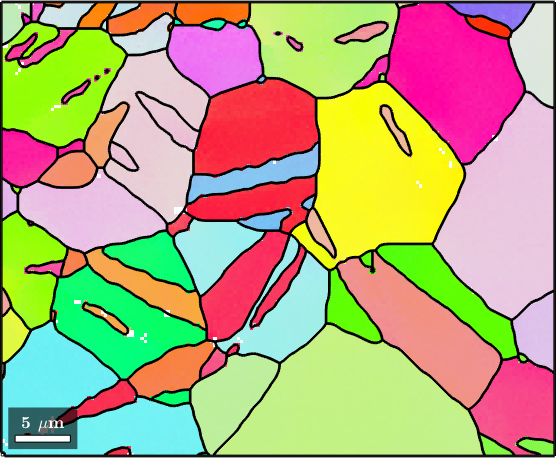

The black network follows the reconstructed grain boundaries. Notice the long, narrow lamellae that cut across the larger magnesium grains. Their morphology suggests twinning, but the following plane analysis tests the crystallographic prediction.

Misorientation angle at grain boundaries

The magnesium tension twins produce a sharp misorientation peak at 86.3 degrees. Separate boundaries above and below 80 degrees to make a first, deliberately coarse comparison. An angle threshold alone does not identify a twin law because different axes can have the same angle.

gB = grains.boundary('indexed');
cond = gB.misorientation.angle > 80*degree;

plot(ebsd,mapColor)
hold on
plot(grains.boundary,'lineWidth',3)
plot(gB(cond),'lineWidth',2,'lineColor','w')
hold off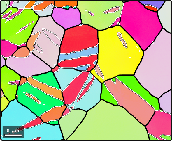

The white traces pick out most of the narrow lamellae. Some high-angle boundaries need not be twins, so this spatial agreement is evidence for the selection rather than a complete classification.

Estimate the two crystal GBNDs

Recovering a three-dimensional distribution from planar traces is a deconvolution. An unconstrained reconstruction can ring around sharp features and become negative. The option 'nonneg' enforces the nonnegative result required for a density.

The 'halfwidth' controls how far each observation is spread in the estimate. See Density Estimation for the resolution--noise trade-off behind this value.

gbnd1 = calcGBND(gB(cond),ebsd,'halfwidth',5*degree,'nonneg');
gbnd2 = calcGBND(gB(~cond),ebsd,'halfwidth',5*degree,'nonneg');

% mark the full family of magnesium tension-twin planes
tp = Miller(1,0,-1,2,CS,'hkil');

% use one colour range so weak structure is not visually amplified
contourf(gbnd1,'colorrange',[0.5 1.5])
mtexTitle('GBND for \(\omega > 80^{\circ}\)')
mtexColorMap parula
annotate(symmetrise(tp),'labeled','backgroundColor','w')
nextAxis
contourf(gbnd2,'colorrange',[0.5 1.5])
mtexTitle('GBND for \(\omega < 80^{\circ}\)')
mtexColorMap parula
mtexColorbar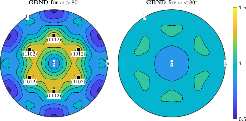

Both panels are normalized so that a value of one is uniform. The common colour range is essential: otherwise automatic scaling would make the nearly uniform right panel appear as structured as the left.

The high-angle distribution has maxima beside the six symmetrically equivalent \(\{10\bar{1}2\}\) planes. These are full-sphere plots, so all six variants are marked. Marking only one plane would single out one maximum for no crystallographic reason. The remaining boundaries stay much closer to one and show no comparable preferred plane.

[highAnglePeak,highAnglePeakPosition] = max(gbnd1);
highAngleSummary = table(highAnglePeak,...
  min(angle(highAnglePeakPosition,symmetrise(tp)))./degree,...
  'VariableNames',{'peakDensity','distanceToTwinPlaneDegree'})

remainingSummary = table(min(gbnd2),max(gbnd2),...
  'VariableNames',{'minimumDensity','maximumDensity'})

highAngleSummary =
  1×2 table
    peakDensity    distanceToTwinPlaneDegree
    ___________    _________________________
      1.3905                5.5946          
remainingSummary =
  1×2 table
    minimumDensity    maximumDensity
    ______________    ______________
       0.86264            1.0868

The peak lies 5.6 degrees from the nearest tension-twin plane. The remaining distribution ranges from 0.86 to 1.09. These values quantify the visual contrast between the panels.

The grain boundary character distribution

The angle split above is intentionally crude. Passing a misorientation as the third argument selects boundaries near that complete relationship and expresses their plane normals consistently. The result is the GBCD slice for that misorientation.

% define the ideal magnesium tension-twin relationship
moriRef = orientation.byAxisAngle(...
  Miller(1,1,-2,0,CS,'uvtw'),86.3*degree,CS,CS);

gbcd = calcGBND(gB,grains,moriRef,...
  'halfwidth',5*degree,'nonneg');

plot(gbcd,'contourf')
mtexTitle('GBCD for the tension twin')
mtexColorMap parula
annotate(symmetrise(tp),'labeled','backgroundColor','w')
mtexColorbar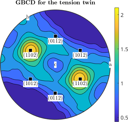

Two of the six \(\{10\bar{1}2\}\) variants carry the maxima. The specimen was deformed, so not every twin variant is equally active. The strongest maximum sits directly on a tension-twin plane.

[twinPeak,twinPeakPosition] = max(gbcd);
twinGBCDSummary = table(twinPeak,...
  min(angle(twinPeakPosition,symmetrise(tp)))./degree,...
  'VariableNames',{'peakDensity','distanceToTwinPlaneDegree'})

twinGBCDSummary =
  1×2 table
    peakDensity    distanceToTwinPlaneDegree
    ___________    _________________________
      2.1012                 1.307

The printed angular distance is 1.3 degrees. Conditioning on the complete misorientation sharpens the habit-plane result compared with the angle-only split.

Three-dimensional data

A triangulated three-dimensional boundary stores its normal directly, so no stereological reconstruction is required. We use the DREAM.3D data set introduced in Three-Dimensional Grains.

grains3 = grain3d.load(...
  fullfile(mtexDataPath,'EBSD','SmallIN100_MeshStats.dream3d'));

% separate internal interfaces from faces on the measured box
allB3 = grains3.boundary;
isInnerFace = all(allB3.grainId > 0,2);
surfaceFaceAreaPercent = 100 * sum(allB3.area(~isInnerFace)) / ...
  sum(allB3.area);
surfaceFaceSummary = table(surfaceFaceAreaPercent,...
  'VariableNames',{'percentOfTotalFaceArea'})
gB3 = allB3(isInnerFace);

surfaceFaceSummary =
  table
    percentOfTotalFaceArea
    ______________________
            22.84

Faces at the surface of the measured volume belong to only one grain. They are the six sides of the measured box, not grain boundaries. They contribute 22.8 percent of the total face area. Their flat, axis-aligned normals would otherwise dominate the specimen GBND.

The specimen GBND

With a three-dimensional boundary as its only argument, calcGBND uses the measured normals in the specimen frame. Each triangular face is weighted by its area.

gbndSpecimen = calcGBND(gB3);

plot(gbndSpecimen,'contourf','upper')
mtexTitle('specimen GBND')
mtexColorMap parula
mtexColorbar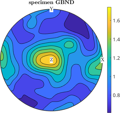

Read this plot in the specimen frame: the strongest maximum lies near Z. It describes a preferred interface direction in the sample, not a crystallographic habit plane. The distribution ranges from 0.61 to 1.74.

specimenSummary = table(min(gbndSpecimen),max(gbndSpecimen),...
  'VariableNames',{'minimumDensity','maximumDensity'})

specimenSummary =
  1×2 table
    minimumDensity    maximumDensity
    ______________    ______________
       0.61127            1.7424

The crystal GBND

Passing the grains as well rotates each measured normal into the crystal frame of the grain beside it. Both sides contribute, and each face keeps its area weight.

gbndCrystal = calcGBND(gB3,grains3);

plot(gbndCrystal,'contourf','complete','upper')
mtexTitle('crystal GBND')
mtexColorMap parula
mtexColorbar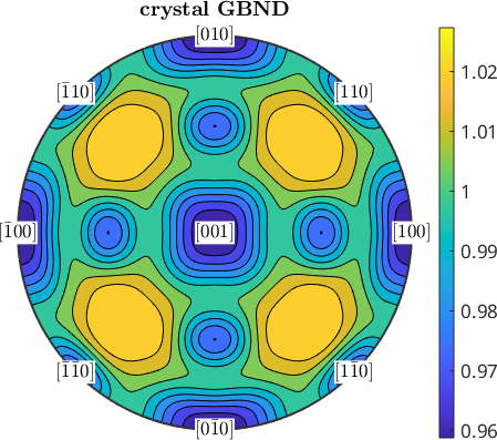

The crystal GBND is almost uniform. Taken over all internal interfaces, this data set has no strong preferred habit plane. Its values range from 0.96 to 1.03.

crystalSummary = table(min(gbndCrystal),max(gbndCrystal),...
  'VariableNames',{'minimumDensity','maximumDensity'})

crystalSummary =
  1×2 table
    minimumDensity    maximumDensity
    ______________    ______________
       0.95879            1.0273

The GBCD in three dimensions

This changes when the distribution is conditioned on the cubic \(\Sigma 3\) misorientation: a 60 degree rotation about a [111] axis. The ten-degree halfwidth below gives the estimator a twenty-degree inclusion window, matching the implementation of the GBCD kernel.

cs3 = grains3.CSList(2);
sigma3 = orientation.byAxisAngle(...
  Miller(1,1,1,cs3),60*degree,cs3,cs3);

% measure a strict Sigma 3 fraction and the broader kernel window
grainInd = grains3.id2ind(gB3.grainId);
ori1 = grains3.meanOrientation(grainInd(:,1));
ori2 = grains3.meanOrientation(grainInd(:,2));
sigma3Deviation = angle(inv(ori1).*ori2,sigma3);
sigma3ToleranceDegree = [5;20];
sigma3FacePercent = zeros(2,1);
sigma3AreaPercent = zeros(2,1);
for k = 1:2
  isSigma3 = sigma3Deviation < sigma3ToleranceDegree(k)*degree;
  sigma3FacePercent(k) = 100 * mean(isSigma3);
  sigma3AreaPercent(k) = 100 * sum(gB3.area(isSigma3)) / sum(gB3.area);
end
sigma3Summary = table(sigma3ToleranceDegree,sigma3FacePercent,...
  sigma3AreaPercent)

gbcd3 = calcGBND(gB3,grains3,sigma3,'halfwidth',10*degree);

plot(gbcd3,'contourf')
mtexTitle('GBCD for \(\Sigma 3\)')
mtexColorMap parula
sigma3Plane = Miller(1,1,1,cs3);
annotate(symmetrise(sigma3Plane),'labeled','backgroundColor','w')
mtexColorbar

sigma3Summary =
  2×3 table
    sigma3ToleranceDegree    sigma3FacePercent    sigma3AreaPercent
    _____________________    _________________    _________________
              5                   26.235               23.249      
             20                   44.815               42.288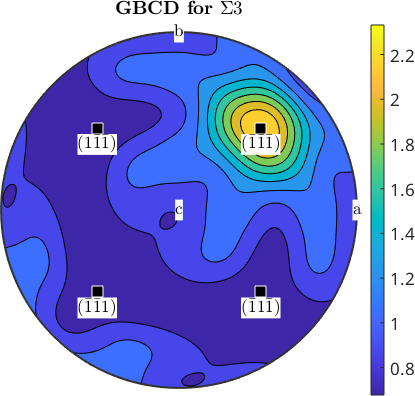

Within 5 degrees of the ideal \(\Sigma 3\) relationship lie 26.2 percent of the internal faces, carrying 23.2 percent of the area. This is the sense in which about a quarter of the inner faces are \(\Sigma 3\) twins. The kernel's 20 degree support admits 44.8 percent of the faces but gives less weight to those farther from the ideal relationship.

Of the four \(\{111\}\) variants, only the variant along the \(\Sigma 3\) rotation axis is strongly populated. These twins are coherent, and the maximum coincides with that boundary plane.

[sigma3Peak,sigma3PeakPosition] = max(gbcd3);
sigma3GBCDSummary = table(sigma3Peak,...
  min(angle(sigma3PeakPosition,symmetrise(sigma3Plane)))./degree,...
  'VariableNames',{'peakDensity','distanceToSigma3PlaneDegree'})

sigma3GBCDSummary =
  1×2 table
    peakDensity    distanceToSigma3PlaneDegree
    ___________    ___________________________
      2.3322                0.0015378

The printed peak distance is less than 0.002 degrees. The all-boundary crystal GBND is nearly uniform, while the \(\Sigma 3\) GBCD is sharply peaked. There is no contradiction: averaging over every misorientation hides a habit that is specific to one boundary character.

Interpreting a stereological estimate

The two-dimensional estimator weights every trace segment by its length. The three-dimensional estimator weights every triangular face by its area. Neither result is a count of physical boundaries or twin domains.

Plane normals are axes: a normal and its negative describe the same unoriented plane. Crystal symmetry adds further equivalent normals, which is why every member of a plane family is annotated above.

A single-section estimate also needs enough differently oriented grains to supply varied crystal-frame views. Strong texture can bias this stereological sampling. Compare orthogonal sections or direct three-dimensional data when the anisotropy is important.

References

Next

This page closes the grain boundary chapter by moving from individual traces to a population of plane normals. Continue with Three-Dimensional Grains to inspect the mesh faces used in the direct calculation, or with Spherical Functions to work with the resulting density objects.

References

- D. M. Saylor and G. S. Rohrer, Determining Crystal Habits from Observations of Planar Sections, Journal of the American Ceramic Society 85 (2002), 2799--2804. This paper develops the stereological precursor for recovering habit planes.
- D. M. Saylor, B. S. El-Dasher, B. L. Adams and G. S. Rohrer, Measuring the Five-Parameter Grain-Boundary Distribution from Observations of Planar Sections, Metallurgical and Materials Transactions A 35 (2004), 1981--1989. This paper extends the method to grain boundary distributions.
- A. P. Sutton and R. W. Balluffi, Interfaces in Crystalline Materials, Clarendon Press, 1995. Chapter 1 develops the five macroscopic boundary parameters and their symmetry.
- V. Randle, Application of EBSD to the Analysis of Interface Planes: Evolution over the Last Two Decades, Journal of Microscopy 230 (2008), 406--413. This review compares direct and stereological interface-plane measurements.
- M. Folwarczny et al., Accurate Grain Boundary Plane Distributions for Textured Microstructures from Stereological Analysis of Orthogonal Two-Dimensional Electron Backscatter Diffraction Orientation Maps, Ultramicroscopy 280 (2026), 114262. This study examines texture bias and the use of orthogonal sections.
- R. Hielscher, R. Kilian, K. Marquardt and E. Wünsche, Efficient Computation of the Grain Boundary Normal Distribution from Two Dimensional EBSD Data, not yet published.