Similarly as periodic functions may be represented as weighted sums of sines and cosines a rotational function \(f\colon \mathcal{SO}(3) \to \mathbb C\) can be written as a series of the form
\[ f({\bf R}) = \sum_{n=0}^N \sum_{k,l = -n}^n \hat f_n^{k,l} \, \mathrm{D}_n^{k,l}({\bf R}) \]
with respect to Fourier coefficients \(\hat f_n^{k,l}\) and the so called Wigner-D functions \(D_n^{k,l}\).
There exists various normalizations for the Wigner-D functions. In MTEX they are \(L_2\) normalized, which means
\[\| D_n^{k,l} \|_2 = 1\]
for all \(n,k,l\). For more information take a look on Wigner-D functions and Integration of SO3Fun's.
We construct an arbitrary ODF which generally is an SO3Fun:
mtexdata dubna
odf = calcODF(pf,'resolution',5*degree,'zero_Range')
pf = PoleFigure (y↑→x)
crystal symmetry : Quartz (321, X||a*, Y||b, Z||c*)
h = (022̅1), r = 72 x 19 points
h = (101̅0), r = 72 x 19 points
h = (101̅1)(011̅1), r = 72 x 19 points
h = (101̅2), r = 72 x 19 points
h = (112̅0), r = 72 x 19 points
h = (112̅1), r = 72 x 19 points
h = (112̅2), r = 72 x 19 points
odf = SO3FunRBF (Quartz → y↑→x)
multimodal components
kernel: de la Vallee Poussin, halfwidth 5°
center: 19848 orientations, resolution: 5°
weight: 1Now we may transform an arbitrary SO3Fun into its Fourier representation using the command SO3FunHarmonic
f = SO3FunHarmonic(odf,'bandwidth',32)f = SO3FunHarmonic (Quartz → y↑→x)
bandwidth: 32
weight: 1Fourier Coefficients
Within the class SO3FunHarmonic rotational functions are represented by their complex valued Fourier coefficients which are stored in the field fun.fhat. They are stored in a linear order, which means f.fhat(1) is the zero order Fourier coefficient, f.fhat(2:10) are the first order Fourier coefficients that form a 3x3 matrix and so on. Accordingly, we can extract the second order Fourier coefficients by
reshape(f.fhat(11:35),5,5)ans =
Columns 1 through 4
0.0000 + 0.0000i 0.0000 + 0.0000i 0.0000 + 0.0000i 0.0000 + 0.0000i
0.0000 + 0.0000i 0.0000 + 0.0000i 0.0000 + 0.0000i 0.0000 + 0.0000i
0.0644 - 0.1745i 0.5731 - 0.3793i 0.8694 + 0.0000i 0.5731 + 0.3793i
0.0000 + 0.0000i 0.0000 + 0.0000i 0.0000 + 0.0000i 0.0000 + 0.0000i
0.0000 + 0.0000i 0.0000 + 0.0000i 0.0000 + 0.0000i 0.0000 + 0.0000i
Column 5
0.0000 + 0.0000i
0.0000 + 0.0000i
0.0644 + 0.1745i
0.0000 + 0.0000i
0.0000 + 0.0000iAs an additional example lets define a harmonic function by its Fourier coefficients \(\hat f_0^{0,0} = 0.5\) and \(\hat f_1 = \left(\begin{array}{rrr} 1 & 4 & 7 \\ 2 & 5 & 8 \\ 3 & 6 & 9 \\ \end{array}\right)\)
f2 = SO3FunHarmonic([0.5,1:9]')

plot(f2)
f2 = SO3FunHarmonic (y↑→x → y↑→x)
isReal: false
bandwidth: 1
weight: 0.5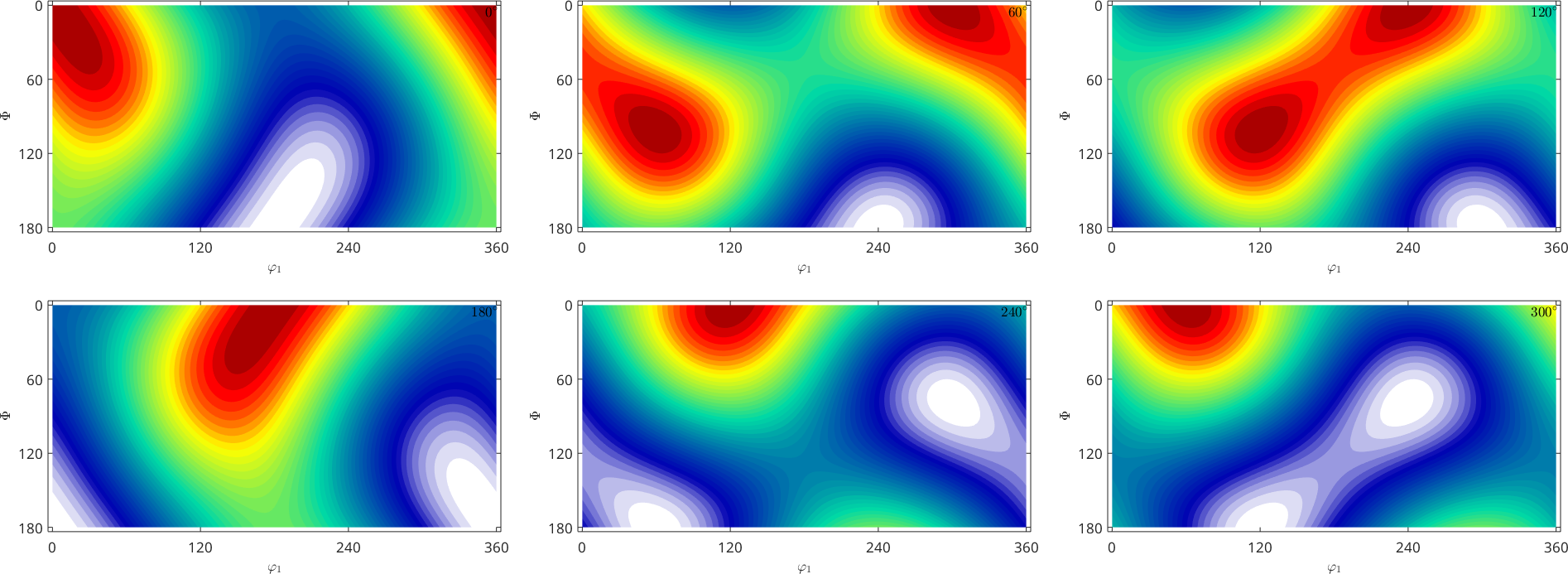
The Fourier coefficients \(\hat f_n^{k,l}\) allow us a complete characterization of the rotational function. They are of particular importance for the calculation of mean macroscopic properties e.g. the second order Fourier coefficients characterize thermal expansion, optical refraction index, and electrical conductivity whereas the fourth order Fourier coefficients characterize the elastic properties of the specimen.
Moreover, the decay of the Fourier coefficients is directly related to the smoothness of the SO3Fun. The decay of the Fourier coefficients might also hint for the presents of a ghost effect. See Ghost Correction.
The decay of the Fourier coefficients is shown in the plot
close all;
plotSpektra(f)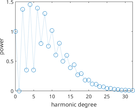
ODFs given by Fourier coefficients
In order to define an ODF by it Fourier coefficients \({\bf \hat{f}}\), they has to be given as a literally ordered, complex valued vector of the form
\[ {\bf \hat{f}} = [\hat{f}_0^{0,0},\hat{f}_1^{-1,-1},\ldots,\hat{f}_1^{1,1},\hat{f}_2^{-2,-2},\ldots,\hat{f}_N^{N,N}] \]
where \(n=0,\ldots,N\) denotes the order of the Fourier coefficients.
cs   = crystalSymmetry('1');    % crystal symmetry
fhat = [1;reshape(eye(3),[],1);reshape(eye(5),[],1)]; % Fourier coefficients
odf = SO3FunHarmonic(fhat,cs)

plot(odf,'sections',6,'silent','sigma')
odf = SO3FunHarmonic (1 → y↑→x)
antipodal: true
bandwidth: 2
weight: 1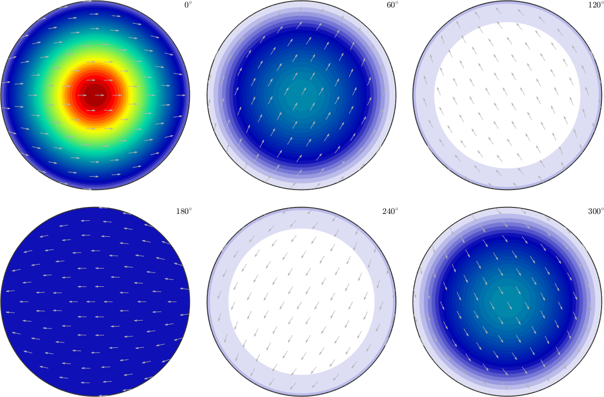
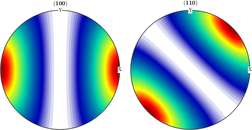
plotPDF(odf,[Miller(1,0,0,cs),Miller(1,1,0,cs)],'antipodal')