The grain reference orientation deviation is the misorientation \(\mathrm{GROD}_{i,j}\) between the orientation \(o_{i,j}\) at position \((i,j)\) and the reference or mean orientation \(o_g\) of the grain the position \((i,j)\) belongs to, i.e.,
\[ \mathrm{GROD}_{i,j} = \mathbf S_{i,j} \cdot \mathrm{inv}(o_g) \cdot o_{i,j} \]
In the above formula the symmetry elements \(\mathbf S_{i,j}\) are chosen to minimize the misorientation angle of \(\mathrm{GROD}_{i,j}\).
Let us demonstrate the computation of the grain reference orientation deviation at the example of a deformed Ferrite specimen. Lets import the data first, reconstruct the grain structure and perform some denoising of the orientation data as the we are going to analyze the misorientation axes which are very noise sensitive.
mtexdata ferrite silent

[grains,ebsd.grainId] = calcGrains(ebsd('indexed'),...
  'threshold',[1*degree, 10*degree],'minPixel',3);

% smooth grain boundaries
grains = smooth(grains,5);

% denoise the orientations
F = halfQuadraticFilter;
ebsd = smooth(ebsd,F,grains,'fill');

plot(ebsd('indexed'),ebsd('indexed').orientations)
hold on
plot(grains.boundary,'lineWidth',2)
hold off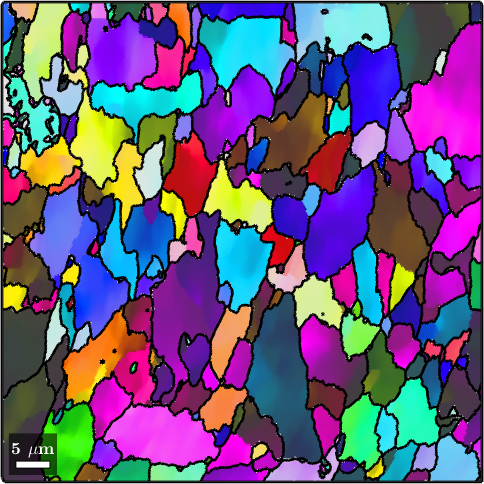
The grain reference orientation deviation is computed by the command calcGROD. It requires the reconstructed grains as second argument and that ebsd.grainId has been set as we did in the above code.
% compute the grain reference orientation deviation
grod = ebsd.calcGROD(grains);
As a first application we simply plot the misorientation angle of the grain reference orientation deviation and overlay it with the subgrain boundaries
% plot the misorientation angle of the GROD
plot(ebsd,grod.angle./degree,'micronbar','off')
mtexColorbar('title',{'misorientation angle in degree'})
mtexColorMap LaboTeX

% overlay grain and sub-grain boundaries
hold on
plot(grains.boundary,'lineWidth',1.5)
plot(grains.innerBoundary,'edgeAlpha',grains.innerBoundary.misorientation.angle / (5*degree))
hold off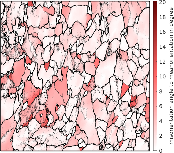
Grain Orientation Spread (GOS)
The grain orientation spread (GOS) is the averaged misorientation angle of the grain reference orientation deviations of each grain. We may compute this average by using the command grainMean.
GOS = grainMean(ebsd, grod.angle, grains);

plot(grains, GOS ./ degree)
mtexColorbar('title','GOS in degree')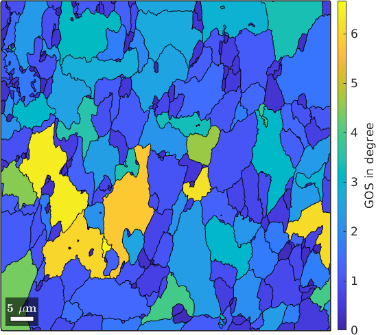
The Misorientation Axis in Crystal Coordinates
When analyzing the misorientation axis of the grain reference orientation deviations we have to distinguish whether we look at them in crystal coordinates or in specimen coordinates. Let's start with the crystal coordinates. In this case we use the command axis to compute the corresponding \((hk\ell)\) values.
Lets first plot the distribution of misorientation axes in the fundamental sector.
axCrystal = grod.axis;

plot(axCrystal,'contourf','fundamentalRegion','antipodal','figSize','small')
mtexColorbar('title','mrd')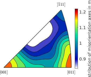
We observe that the distribution is very uniform and there is no preferred misorientation axes. Lets have a look at the spatial distribution of the misorientation axes. To this end we firs have to define a directional color key.
colorKey = HSVDirectionKey(ebsd.CS,'antipodal');

plot(colorKey,'figSize','small')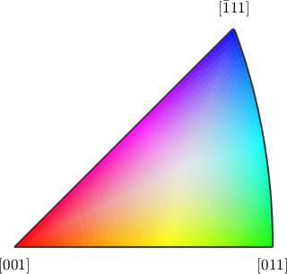
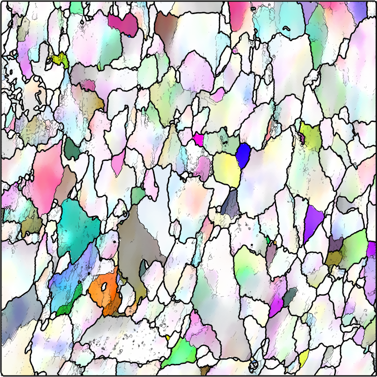
When plotting the misorientation axis we use the misorientation angle as transparency value to fade out low angles misorientations to white.
% compute the color from the misorientation axis
color = colorKey.direction2color(axCrystal);

% and set the transparency from the misorientation angle
alpha = min(grod.angle/degree/7.5,1);

% plot the data
plot(ebsd,color,'micronbar','off','faceAlpha',alpha,'figSize','large')

hold on
plot(grains.boundary,'lineWidth',2)
plot(grains.innerBoundary,'edgeAlpha',grains.innerBoundary.misorientation.angle / (5*degree))
hold off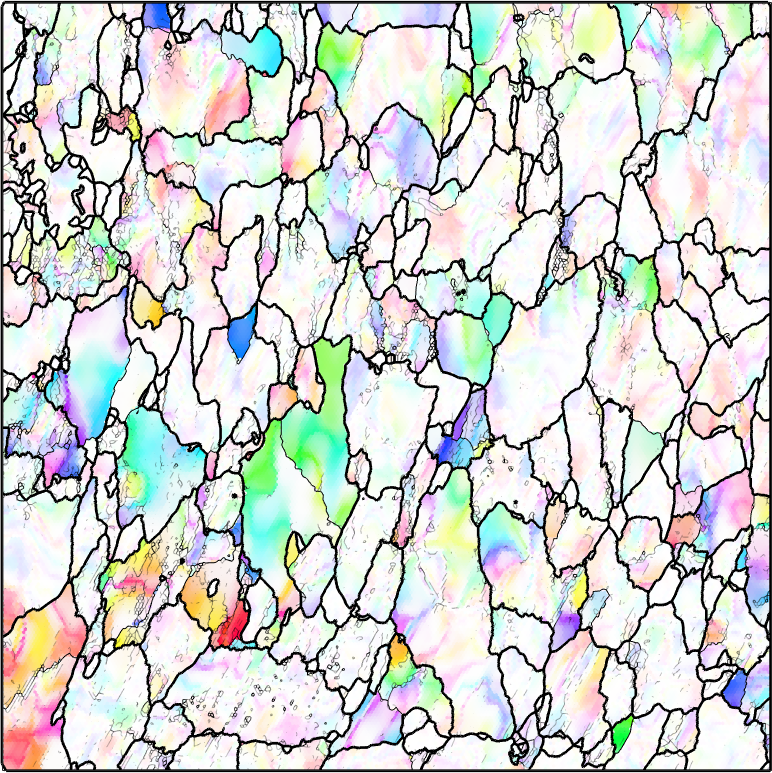
The misorientation axis in crystal coordinates can be related to active slip systems. See: V. Tong, E. Wielewski, B. Britton Characterization of slip and twinning in high rate deformed zirconium with electron backscatter diffraction, 2018.
TODO: explain this at some new documentation page
The Misorientation Axis in Specimen Coordinates
The misorientation axis in specimen coordinates is computed by applying the EBSD orientations to the the misorientation axes in crystal coordinates. It is important to use here the option 'noSymmetry'.
axSpecimen = ebsd.orientations .* grod.axis('noSymmetry');

plot(axSpecimen,'contourf','fundamentalRegion','antipodal','halfwidth',2.5*degree)
mtexColorbar('title','distribution of misorientation axes in mrd')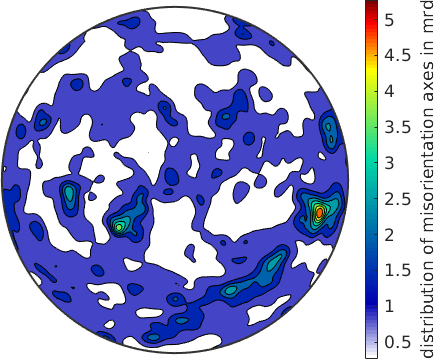
When looking at the distribution of the misorientation axes in specimen coordinates we observe some strongly preferred directions.
As the misorientation axes in specimen coordinates have no symmetry at all (not even antipodal symmetry) we may use a full color key to colorize them
colorKey = HSVDirectionKey;

plot(colorKey,'figSize','small')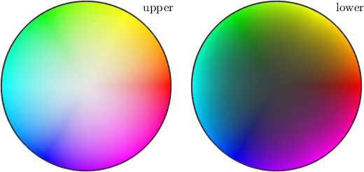
The spatial plot of the misorientation axes in crystal coordinates follows the same lines as the plot in specimen coordinates.
% compute color and transparency
omega = min(grod.angle/degree/7.5,1);
color = colorKey.direction2color(axSpecimen);

% plot the data
plot(ebsd,color,'micronbar','off','FaceAlpha',omega,'figSize','large')

hold on
plot(grains.boundary,'lineWidth',2)
plot(grains.innerBoundary,'edgeAlpha',grains.innerBoundary.misorientation.angle / (5*degree))
hold off

%omega = min(grod.angle/degree/7.5,1);
%color = colorKey.direction2color(axSpecimen,'grayValue',omega);