
Grain segmentation correctly identifies a twin domain as a grain: it is a phase-homogeneous, spatially connected region of EBSD measurements. For an analysis of the grain before twinning, however, that domain belongs to its host. Merging removes the selected internal boundaries and reconstructs this parent-grain footprint.
In parent-phase reconstruction, merging is the second of two distinct steps. The child grains are first transformed to candidate parent orientations and only then merged where those candidates are compatible. See Grain Graph Based Reconstruction for that complete workflow.
This page uses deformation twins in magnesium. It assumes familiarity with grain reconstruction, grain IDs, and boundary misorientations.
close all;

% load the example in its specimen plotting frame
plottingConvention.default('y↑→x');
mtexdata twins silent

% reconstruct and smooth the grains
[grains,ebsd] = calcGrains(ebsd,'angle',5*degree,'minPixel',3);
grains = smoothBoundary(grains,5);
grains = grains('indexed');

% compute the mean-orientation colours without printing a colour-key notice
colorKey = ipfColorKey(grains);
grainColor = colorKey.orientation2color(grains.meanOrientation);
plot(grains,grainColor)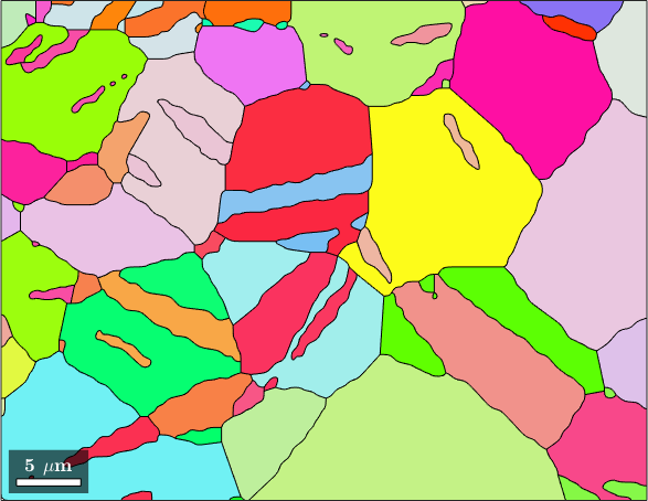
The narrow lamellae have mean-orientation colours unlike their surrounding grains. Their morphology suggests twins, but morphology alone does not establish a twin relationship.
Select candidate twin boundaries
A twin law maps two pairs of crystallographic directions onto each other. orientation.map constructs that complete relationship. Comparing complete misorientations is more selective than comparing their rotation angles alone.
% define the ideal twinning misorientation
CS = grains.CS;
twinning = orientation.map(Miller(0,1,-1,-2,CS),Miller(0,-1,1,-2,CS),...
  Miller(2,-1,-1,0,CS),Miller(2,-1,-1,0,CS));

% extract magnesium-to-magnesium grain boundaries
gB = grains.boundary('Magnesium','Magnesium');

% select segments within 5 degrees of the twin law
isTwinning = angle(gB.misorientation,twinning) < 5*degree;
twinBoundary = gB(isTwinning)

% report how much of the sampled boundary network passed the test
boundarySummary = table(length(gB),length(twinBoundary),...
  100*length(twinBoundary)/length(gB),...
  'VariableNames',{'MgMgSegments','candidateTwinSegments','percent'})

% overlay the candidate twin boundaries
hold on
plot(twinBoundary,'linecolor','w','linewidth',4,...
  'displayName','candidate twin boundary')
hold off
twinBoundary = grainBoundary (y↑→x)
Segments length mineral 1 mineral 2
1406 356 µm Magnesium Magnesium
boundarySummary =
1×3 table
MgMgSegments candidateTwinSegments percent
____________ _____________________ _______
2696 1406 52.151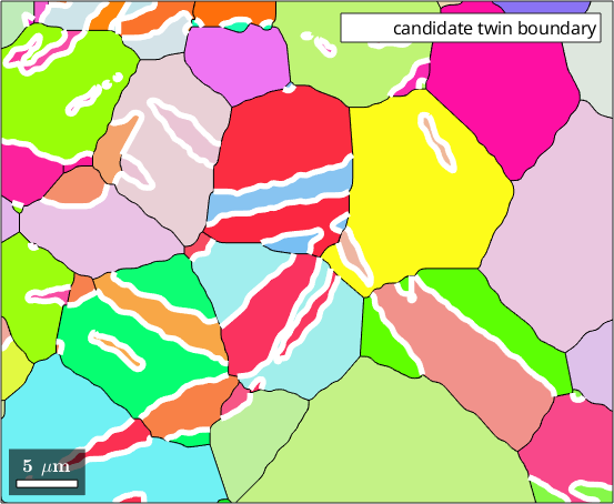
The white traces follow the narrow lamellae. With this boundary sampling, 1406 of 2696 magnesium-to-magnesium segments pass the five-degree test. A segment count is not a count of physical twins, and smoothing or resampling the same traces can change it. The tolerance is also an analyst choice: these are candidate twin boundaries, not proof of the mechanism or of which side is the parent. Inferring Twin Boundaries develops those limitations.
Merging along selected boundaries
merge joins the grains on both sides of every supplied boundary. It treats the selected boundaries as connections in a graph and merges each connected component. The operation is therefore transitive: if A is joined to B and B to C, all three become one grain. One false connecting boundary can consequently fuse a much larger parent than expected.
[mergedGrains,parentId] = merge(grains,twinBoundary);

mergeSummary = table(length(grains),length(mergedGrains),...
  'VariableNames',{'grainsBefore','grainsAfter'})

% overlay the reconstructed parent-grain boundaries
hold on
plot(mergedGrains.boundary,'linecolor','k','linewidth',2.5,...
  'linestyle','-','displayName','merged grains')
hold off
mergeSummary =
1×2 table
grainsBefore grainsAfter
____________ ___________
91 28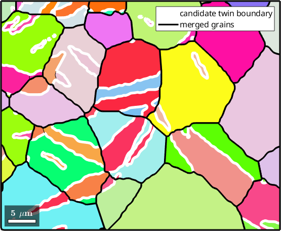
The 91 segmented grains have become 28 merged grains. Black lines are the reconstructed parent-grain outlines. Each white trace that no longer has a black line on it is now internal to one merged grain.
Keeping track of the child grains
The second output, parentId, has one entry for every grain in grains. parentId(k) is the ID of the merged grain that contains grains(k). This is the same kind of bookkeeping that ebsd.grainId provides between measurements and grains; it is a mapping of persistent IDs, not a list position.
selectedParentId = mergedGrains(16).idselectedParentId =
16The following object summary lists the child grains assigned to merged grain 16.
childs = grains(parentId == selectedParentId)childs = grain2d (y↑→x)
Phase Grains Pixels Mineral Symmetry Color
1 9 456 Magnesium 6/mmm LightSkyBlue
boundary segments: 200 (56 µm)
inner boundary segments: 0 (0 µm)
triple points: 15
Id Phase Pixels meanRotation GOS
11 1 18 (132°,46°,215°) 0.0093
15 1 7 (66°,157°,185°) 0.0081
22 1 94 (29°,68°,224°) 0.016
24 1 6 (31°,69°,225°) 0.02
26 1 56 (63°,154°,181°) 0.011
33 1 26 (30°,70°,224°) 0.013
35 1 4 (58°,152°,237°) 0.012
36 1 125 (30°,67°,224°) 0.015
37 1 120 (67°,158°,185°) 0.018Which child domains are twins
Merging establishes which domains belong together. It does not identify the original host or the twin. One simple rule works while twins occupy less area than their host: cluster each parent's child orientations and label the largest orientation cluster by area as the original grain.
% cache the child-grain areas
gArea = grains.area;

% classify the smaller orientation clusters as twin domains
isTwin = true(grains.length,1);
for i = 1:mergedGrains.length

  % find the children of this merged-grain ID
  parent = mergedGrains(i).id;
  childInd = find(parentId == parent);

  % cluster children with similar mean orientations
  [fId,~] = calcCluster(grains.meanOrientation(childInd),'maxAngle',...
    15*degree,'method','hierarchical','silent');

  % find the orientation cluster with the largest total area
  clusterArea = accumarray(fId,gArea(childInd));
  [~,fParent] = max(clusterArea);
  isTwin(childInd(fId == fParent)) = false;
end

% report the mapped-area fraction assigned to twins
twinAreaPercent = 100*sum(area(grains(isTwin)))/sum(area(grains))

% visualize the classification
close all
plot(grains(~isTwin),'FaceColor','darkgray','displayName','not twin')
hold on
plot(grains(isTwin),'FaceColor','red','displayName','twin')
plot(mergedGrains.boundary,'linecolor','k','linewidth',2,...
  'linestyle','-','displayName','merged grains')
mtexTitle('twin classification')
hold off
twinAreaPercent =
16.6397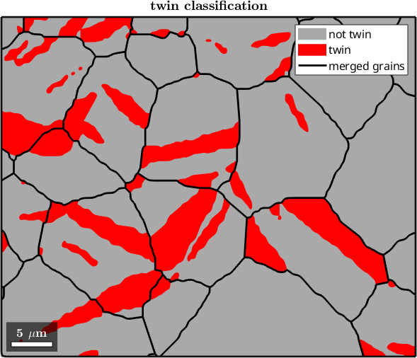
The rule assigns 17 percent of the mapped area to twins. The red domains are lamellae inside the grey hosts, which is a useful spatial check on the classification. The rule fails if a twin consumes more than half of its host. This map alone cannot reveal that history.
Properties of the merged grains
A merged grain receives a new shape and the summed pixel count. Other grain properties have no universal merge rule. In particular, directly averaging host and twin orientations usually does not recover the host orientation, so the 'calcMeanOrientation' option is not appropriate for this example. The intended physical quantity must determine how each property is carried from children to parents.
For grain orientation spread (GOS), parentId supplies the groups to accumarray. An unweighted mean gives every child grain one vote.
% compute an unweighted child-grain mean for each parent
unweightedGOS = accumarray(parentId,grains.GOS,size(mergedGrains),@mean);
mergedGrains.prop.GOS = unweightedGOS;

% compare child and unweighted parent values
close all
plot(grains,grains.GOS./degree)
hold on
plot(mergedGrains.boundary,'lineColor','white','lineWidth',2)
mtexTitle('child-grain GOS')

nextAxis(1,2)
plot(mergedGrains,unweightedGOS./degree)
mtexTitle('unweighted merged GOS')
setColorRange([0,1.5])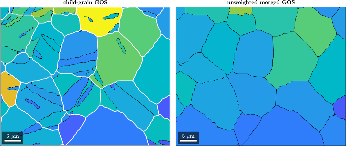
This mean counts a two-pixel twin as much as the grain that contains it. That is rarely the intended statistic. Weighting each child by area gives each measured part of the parent equal influence.
% cache GOS and area for the weighted accumulation
childGOS = grains.GOS;
childArea = grains.area;

% compute the area-weighted child-grain mean for each parent
weightedGOS = accumarray(parentId,1:length(grains),size(mergedGrains),...
  @(id) nanmeanWeights(childGOS(id),childArea(id)));
mergedGrains.prop.GOS = weightedGOS;

nextAxis(1,3)
plot(mergedGrains,weightedGOS./degree)
mtexTitle('area-weighted merged GOS')
mtexColorbar
setColorRange([0,1.5])

gosSummary = table(nnz(weightedGOS > unweightedGOS),length(mergedGrains),...
  max(weightedGOS-unweightedGOS)./degree,...
  'VariableNames',{'weightedValueHigher','parents','maximumIncreaseDegree'})
gosSummary =
1×3 table
weightedValueHigher parents maximumIncreaseDegree
___________________ _______ _____________________
14 28 0.58077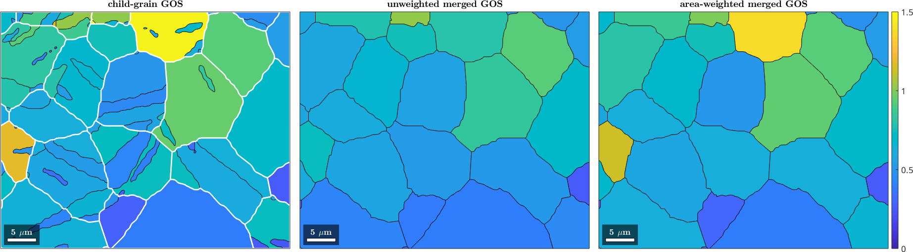
The two parent maps differ in both directions. The weighted value is larger in 14 of the 28 parents, by as much as 0.6 degrees. In those parents the larger children carry the higher GOS values, while small twins pull the unweighted mean down. More generally, orientation spread can depend on grain size, so the weighting rule must be reported.
Pointing EBSD measurements at the merged grains
The EBSD measurements still carry the grainId values from the original segmentation. Those IDs refer to a different grain list after merging. Indexing ebsd with a merged grain therefore selects the wrong measurements without raising an error.
targetMergedGrain = mergedGrains('id',22);
staleMeasurements = ebsd(targetMergedGrain);
staleColor = colorKey.orientation2color(staleMeasurements.orientations);

close all
plot(targetMergedGrain.boundary,'linewidth',2)
hold on
plot(staleMeasurements,staleColor)
hold off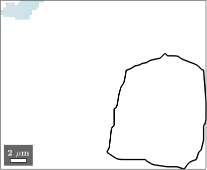
The coloured measurements do not fill the outlined merged grain. They are the measurements whose old grainId happens to equal the new ID 22. Replace every indexed measurement's old grain ID by the parent ID of its original grain.
% copy the EBSD data so the original mapping remains available
ebsd_merged = ebsd;

% map old grain IDs to indices in grains, then from children to parent IDs
ebsd_merged('indexed').grainId = ...
  parentId(grains.id2ind(ebsd('indexed').grainId));

correctedMeasurements = ebsd_merged(targetMergedGrain);
correctedColor = colorKey.orientation2color(correctedMeasurements.orientations);
The same lookup now returns the measurements inside the outline. Updating grainId is essential whenever subsequent EBSD analysis uses the merged grains.
plot(correctedMeasurements,correctedColor)
hold on
plot(targetMergedGrain.boundary,'linewidth',3)
hold off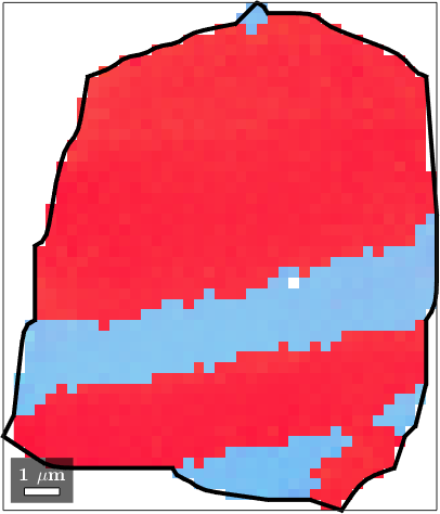
References
- F. Bachmann, R. Hielscher, and H. Schaeben, Grain Detection from 2d and 3d EBSD Data--Specification of the MTEX Algorithm, Ultramicroscopy 111 (2011), 1720--1733. This paper derives the grain and boundary network on which merging operates.
- J. W. Christian and S. Mahajan, Deformation Twinning, Progress in Materials Science 39 (1995), 1--157. This review develops the crystallography and mechanisms of deformation twins.
- W. Pantleon, W. He, T. O. Johansson, and C. Gundlach, Orientation Inhomogeneities within Individual Grains in Cold-Rolled Aluminium Resolved by Electron Backscatter Diffraction, Materials Science and Engineering A 483--484 (2008), 668--671. This paper discusses orientation spread and its dependence on grain size.
- ASTM E2627-13(2019), Standard Practice for Determining Average Grain Size Using Electron Backscatter Diffraction (EBSD) in Fully Recrystallized Polycrystalline Materials. Its scope is fully recrystallized materials, but it shows why boundary and grain definitions must be stated when merged grains enter a size analysis.
Next
Continue with Inferring Twin Boundaries when the twin law must be inferred from the data. For a phase transformation, see Grain Graph Based Reconstruction for the transform-then-merge workflow.
Citing this page.
This page is part of the documentation of
MTEX, a free and open
source MATLAB toolbox for analyzing and modeling crystallographic textures.
It was written by The MTEX Developers and is published at
https://mtex-toolbox.github.io/GrainMerge.html.
If you use MTEX, or reuse text or figures from this page, in your research,
please cite
F. Bachmann, R. Hielscher, H. Schaeben: Texture Analysis with MTEX - Free and Open Source Software Toolbox, Solid State Phenomena 160 (2010), 63-68. 10.4028/www.scientific.net/SSP.160.63
BibTeX
@article{bachmann2010mtex,
  author  = {F. Bachmann and R. Hielscher and H. Schaeben},
  title   = {Texture Analysis with MTEX - Free and Open Source Software Toolbox},
  journal = {Solid State Phenomena},
  volume  = {160},
  pages   = {63-68},
  year    = {2010},
  doi     = {10.4028/www.scientific.net/SSP.160.63},
  url     = {https://doi.org/10.4028/www.scientific.net/SSP.160.63}
}
Other papers describing specific MTEX methods are listed under Publications — please cite the one that best fits your application. The MTEX source code is licensed under the GNU General Public License v2.0; the text and figures of this documentation are licensed under CC BY 4.0, which permits reuse — including by automated systems — provided The MTEX Developers and this page are credited.