Operations with Three-Dimensional Grains

The Three-Dimensional EBSD Analysis overview distinguishes volume measurements from the grain3d surface representation. This page shows how to cut those grains into a planar map, replace polygonal faces by triangles, and rotate geometry together with orientation.

The examples use the synthetic tessellation introduced on the Neper Interface page. The preceding Properties of Three-Dimensional Grains page explains the volume, surface, and face properties used below.

plottingConvention.default('y↑→x');

Load the example microstructure

% Assign trigonal quartz symmetry, as on the Neper Interface page.
cs = crystalSymmetry.load('quartz.cif');
tessFile = fullfile(mtexDataPath,'Neper','my100grains.tess');
grains = grain3d.load(tessFile,'CS',cs)

plot(grains,grains.meanOrientation,'micronbar','off','edgeAlpha',0.1)
setCamera(plottingConvention.default3D)

grains = grain3d (y↑→x)
 
 Phase  Grains  Volume  Mineral  Symmetry  Crystal reference frame
     2    1000      32   Quartz       321        X||a*, Y||b, Z||c
 
 boundary faces: 7131
 
 Properties: meanRotation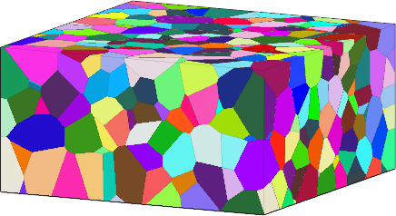

Each colour represents the mean orientation of one grain. The outer faces hide most of the grains inside the tessellated volume, which is why a planar section answers a different question from this surface view.

Cut one planar section

Three-Dimensional Grains introduces planar sectioning and the grain2d result. The direct form of slice used here specifies the plane by a normal N and any point P0 in the plane.

% Point through which the plane passes.
P0 = grains.midPoint;

% Plane normal.
N = vector3d(1,-1,1);

grainSlice = grains.slice(N,P0)

plot(grainSlice,grainSlice.meanOrientation,'micronbar','off')
setCamera(plottingConvention.default3D)

grainSlice = grain2d (y↑→x)
 
 Phase  Grains  Pixels  Mineral  Symmetry         Color
     2     164     164   Quartz       321  LightSkyBlue
 
 boundary segments: 495 (92 µm)
 inner boundary segments: 0 (0 µm)
 triple points: 281
 
 Properties: meanRotation, Id3d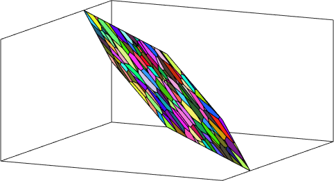

The slice is still drawn in the three-dimensional scene. From the default viewpoint it is seen obliquely. A plotting convention with N pointing out of the screen gives the face-on view a microscope would have.

sectionView = plottingConvention;
sectionView.outOfScreen = N;
sectionView.north = zvector;
setCamera(sectionView)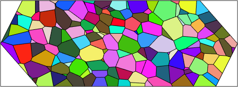

The polygons are cuts through grains, not complete grains. A grain that is large in this section may occupy little volume, and a large grain can be missed when the plane does not intersect it.

The returned Id3d property records the array position of each parent grain in the original collection. Use it to recover the full polyhedra that produced selected section polygons.

parentIds = unique(grainSlice.Id3d);
parentGrains = grains(parentIds);

newMtexFigure('layout',[1,2]);
plot(grainSlice,grainSlice.meanOrientation,'micronbar','off')
setCamera(sectionView)
mtexTitle('Planar sections')

nextAxis
plot(parentGrains,parentGrains.meanOrientation,'micronbar','off','edgeAlpha',0.1)
setCamera(plottingConvention.default3D)
mtexTitle('Parent grains')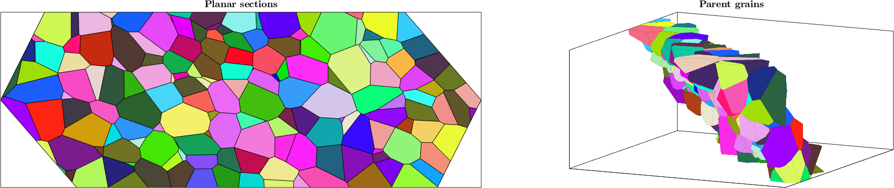

The left panel contains only the section polygons. The right panel shows their parent polyhedra extending on both sides of the cutting plane.

How representative is a grain's section size?

Compare each section's equal-area-circle diameter with the equivalent- sphere diameter of its parent. Id3d is an array position in the collection passed to slice, not a persistent grain ID; retain that collection until the correspondence has been used.

dSection = 2*sqrt(grainSlice.area/pi);
dParent = (6*grains(grainSlice.Id3d).volume/pi).^(1/3);
figure
scatter(dParent,dSection,24,'filled')
hold on
limit = max([dParent;dSection]);
plot([0 limit],[0 limit],'k--')
hold off
axis equal
xlabel('parent equivalent-sphere diameter (length units)')
ylabel('section equal-area-circle diameter (length units)')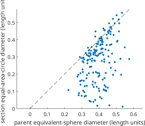

The dashed line marks equal diameters. The spread reflects both the cutting position and grain shape. It is not a calibration curve: a differently placed plane samples different grains, and elongated grains can have section diameters above the line.

Compare several parallel sections

Several slices require several calls to slice. Drawing horizontal cuts together shows how little of the volume any single section represents.

figure
N = vector3d.Z;
zLevels = linspace(min(grains.V.z),max(grains.V.z),7);
for k = zLevels(2:end-1)

  grainSlice = grains.slice(N,vector3d(0,0,k));
  plot(grainSlice,grainSlice.meanOrientation)
  % Interactive selection cannot combine grain2d objects from different planes.
  rmappdata(gca,'grains')
  hold on

end
hold off
setCamera(plottingConvention.default3D)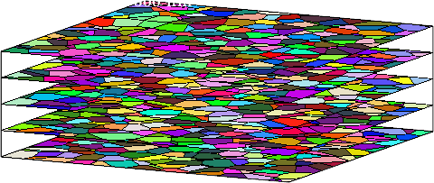

Follow one colour from slice to slice. A grain that is large in one section may be absent from the next.

Triangulate polygonal faces

The faces of these grains are polygons with many vertices. Some computations are much faster on triangles. triangulate returns equivalent grains whose polygonal faces have been divided into triangles.

selectedGrains = grains(20:21);
grainsTri = selectedGrains.triangulate

full([sum(selectedGrains.numFaces), sum(grainsTri.numFaces)])

plot(grainsTri,grainsTri.meanOrientation,'micronbar','off','edgeAlpha',0.1)
setCamera(plottingConvention.default3D)

grainsTri = grain3d (y↑→x)
 
 Phase  Grains  Volume  Mineral  Symmetry  Crystal reference frame
     2       2   0.081   Quartz       321        X||a*, Y||b, Z||c
 
 boundary faces: 88
 
 Id   Phase   Pixels             meanRotation
 20       2        1   (234.8°,161.9°,233.5°)
 21       2        1     (6.2°,129.9°,130.9°)
 
ans =
    28    88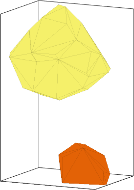

The face count increases while the displayed shape is unchanged: the new triangles cover the same boundary polygons. Triangulation changes the mesh representation, not the physical grains or their stored mean orientations.

Rotate geometry and orientation together

rotate turns grains in space. By default it rotates both things a grain carries: its shape and its orientation. Rotating only one of them would describe a different specimen rather than the same specimen seen differently.

rot = rotation.byAxisAngle(vector3d(1,1,1),30*degree);
grainsRotated = rot * grains;

plot(grainsRotated,grainsRotated.meanOrientation,'micronbar','off','edgeAlpha',0.1)
setCamera(plottingConvention.default3D)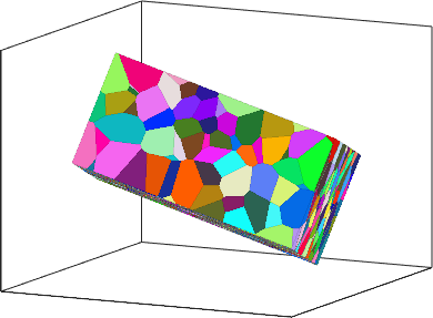

The shape has turned about the coordinate origin, and the colours change. An IPF colour says which crystal direction points along a fixed specimen axis. The same rotation is applied to all orientations; symmetry-reduced orientation differences need not equal that rotation angle. A rigid rotation preserves the relation between grains, while changing their relation to the coordinate axes.

The method form provides a 'center' option when the spatial rotation should use a point other than the origin.

rotationCenter = grains.midPoint;
grainsAboutCenter = rotate(grains,rot,'center',rotationCenter);

Rotate only one part of the data

Two flags deliberately decouple geometry from orientation. The names say which values are kept fixed, not which values are rotated.

For example, the first command below turns the vertices while retaining the orientation values. The second changes the orientations while retaining the vertices.

geometryOnly = rotate(grains,rot,'keepEuler');
orientationOnly = rotate(grains,rot,'keepXY');

These flags are useful when geometry and orientation require separate corrections. They do not represent a rigid rotation of the whole specimen. The 'center' option affects only a spatial rotation, so it has no effect when 'keepXY' leaves the geometry unchanged.

Function reference

References