Bingham Distribution

Theory

The Bingham distribution has the density function

\[ f(g;K,U) = _1\!F_1 \left(\frac{1}{2},2,K \right)^{-1} \exp \left\{ g^T UKU g \right\},\qquad g\in S^3, \]

where \(U\) is an \(4 \times 4\) orthogonal matrix with unit quaternions \(u_{1,..,4}\in S^3\) in the columns and \(K\) is a \(4 \times 4\) diagonal matrix with the entries \(k_1,..,k_4\) describing the shape of the distribution. \(_1F_1(\cdot,\cdot,\cdot)\) is the hypergeometric function with matrix argument normalizing the density.

The shape parameters \(k_1 \ge k_2 \ge k_3 \ge k_4\) give

The general setup of the Bingham distribution in MTEX is done as follows

cs = crystalSymmetry('1');

kappa = [100 90 80 0];   % shape parameters
U     = eye(4);          % orthogonal matrix

odf = BinghamODF(kappa,U,cs)

odf = SO3FunBingham (1 → y↑→x)
 
  kappa: 100 90 80 0
  weight: 1

Lets visualize the ODF as pole figures

h = Miller({0,0,1},{1,0,0},{1,1,1},cs);
plotPDF(odf,h,'antipodal','silent','layout',[1 3]);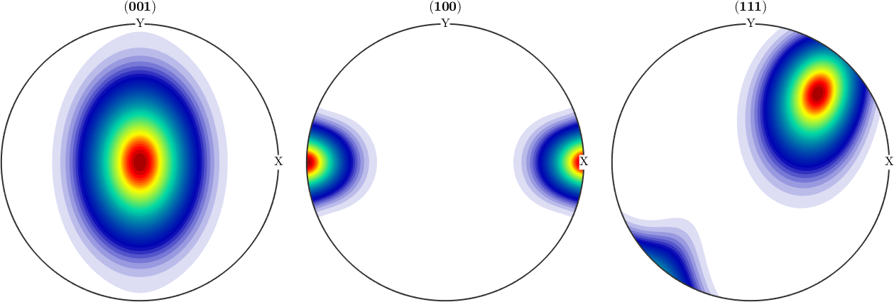

and in Euler angle space

plot(odf,'sections',6)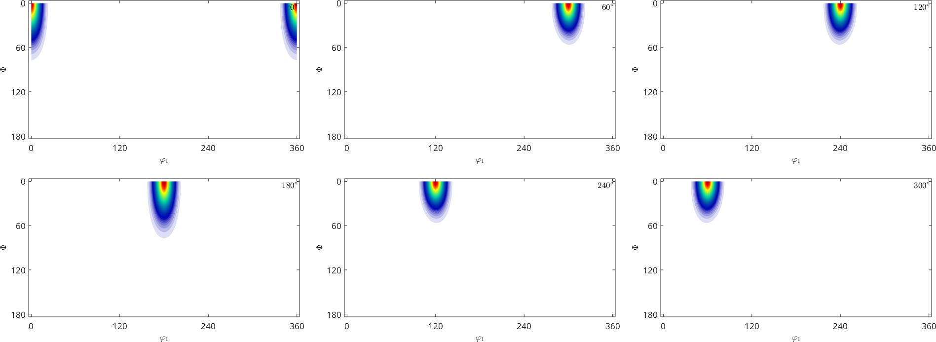

Estimating the parameters of a Bingham distribution

The importance of the Bingham distribution is that it is a quite low dimensional model for an orientation distribution function that still is flexible enough to represent different kinds of textures like fibers and unimodal distributions. Furthermore, we may estimate Bingham distribution from a set of individual orientations, coming e.g. from an EBSD measurement or a plasticity simulation. In contrast to kernel density estimation estimating the parameters of the Bingham distributions requires much less data. Lets demonstrate the process of fitting a Bingham ODF to experimental data. To this end we start with a randomly aligned fibre ODF

odfTrue = fibreODF(fibre.rand(cs));

plotPDF(odfTrue,h,'antipodal','silent')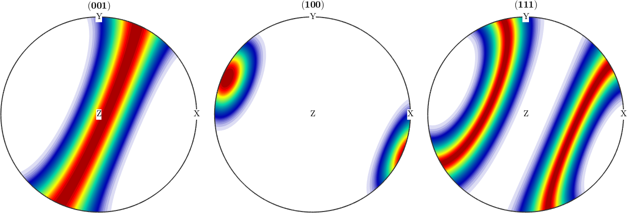

Next we use this fibre ODF to simulate only 1000 random orientations using the command discreteSample

ori = discreteSample(odfTrue,1000);
plot(ori,'add2all','MarkerEdgeColor','k',...
  'MarkerSize',5,'MarkerFaceColor','none','MarkerEdgeAlpha',0.2)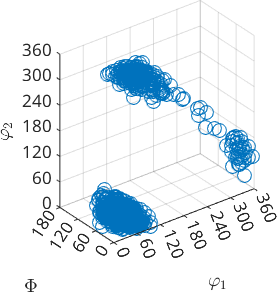

To those simulated orientation data we can now fit a Bingham distribution using the command calcBinghamODF

odf = calcBinghamODF(ori)

plotPDF(odf,h,'antipodal','silent')

odf = SO3FunBingham (1 → y↑→x)
 
  kappa: 0 28 198 198
  weight: 1

We observe an almost perfect fit between the original fibre ODF and the Bingham distribution estimated from only 1000 randomly drawn orientations.

Specific Bingham distributions

In the following we present the three corner cases of the Bingham distribution: the unimodal distribution, the fibre distribution, and the spherical distribution.

The unimodal case A unimodal Bingham distribution with reference orientation oriRef and kappa=40 is constructed by

% a modal orientation
cs = crystalSymmetry('321');
oriRef = orientation.byEuler(45*degree,0*degree,0*degree,cs);

% the corresponding Bingham ODF
odf = BinghamODF(20,oriRef)

plot(odf,'sections',6,'silent','contourf','sigma')

odf = SO3FunBingham (321 → y↑→x)
 
  kappa: 20 0 0 0
  weight: 1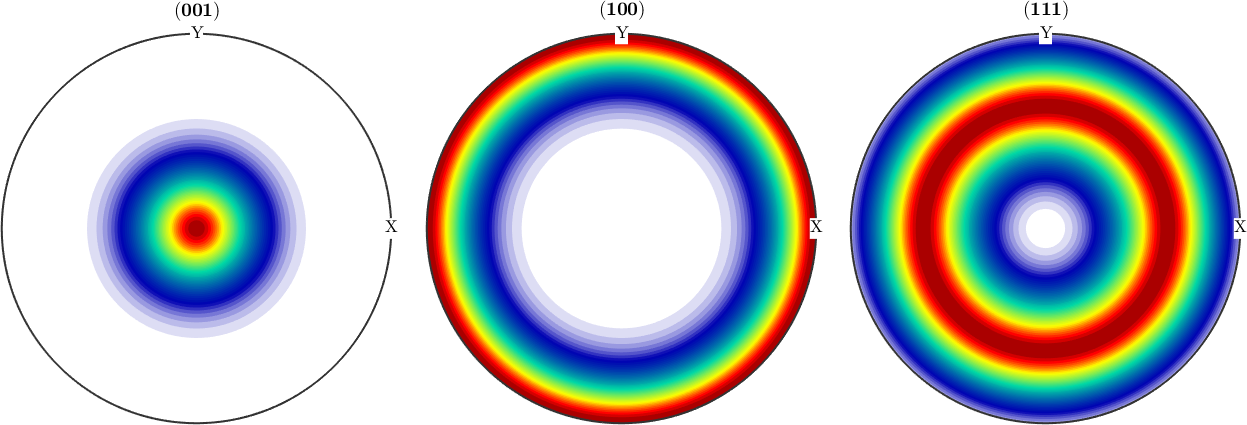

The fibre case For a fibre symmetric Bingham distribution we simply specify the fibre and the first kappa parameter. The first two kappa parameters are allways equal while the third and fourth are zero.

f = fibre.rand(cs);
odf = BinghamODF(20,f)

plot(odf,'sections',6,'silent','sigma')

odf = SO3FunBingham (321 → y↑→x)
 
  kappa: 20 20 0 0
  weight: 1

The spherical case The spherical case is characterized by the fact that we have 3 equal non zero kappa coefficients.

odf = BinghamODF([10,10,10],quaternion(eye(4)),cs)

plot(odf,'sections',6,'silent','sigma');

odf = SO3FunBingham (321 → y↑→x)
 
  kappa: 10 10 10 0
  weight: 1

TODO

where U is the orthogonal matrix of eigenvectors of the orientation tensor and kappa the shape parameters associated with the U.

next, we test the different cases of the distribution on rejection

%T_spherical = bingham_test(ori_spherical,'spherical','approximated');
%T_oblate    = bingham_test(ori_spherical,'prolate',  'approximated');
%T_prolate   = bingham_test(ori_spherical,'oblate',   'approximated');

%t = [T_spherical T_oblate T_prolate]

The spherical test case failed to reject for some level of significance, hence we would dismiss the hypothesis prolate and oblate.

%df_spherical = BinghamODF(kappa,U,cs)

%plotPDF(odf_spherical,h,'antipodal','silent')

Prolate case and fiber distribution

The prolate case corresponds to a fiber.

%odf_prolate = fibreODF(fibre.rand(cs),'halfwidth',20*degree)

%plotPDF(odf_prolate,h,'upper','silent')

As before, we generate some random orientations from a model odf. The shape in an axis/angle scatter plot reminds of a cigar

%ori_prolate = discreteSample(odf_prolate,10000);

%plot(ori_prolate,'axisAngle')

We estimate the parameters of the Bingham distribution

%odf = calcBinghamODF(ori_prolate)

%plotPDF(odf,h,'upper','silent')

and test on the three cases

%T_spherical = bingham_test(ori_prolate,'spherical','approximated');
%T_oblate    = bingham_test(ori_prolate,'prolate',  'approximated');
%T_prolate   = bingham_test(ori_prolate,'oblate',   'approximated');

%t = [T_spherical T_oblate T_prolate]

The test clearly rejects the spherical and prolate case, but not the prolate. We construct the Bingham distribution from the parameters, it might show some skewness

%odf_prolate = BinghamODF(kappa,U,cs)

%plotPDF(odf_prolate,h,'antipodal','silent')

Oblate case

The oblate case of the Bingham distribution has no direct counterpart in terms of texture components, thus we can construct it straightforward

%odf_oblate = BinghamODF([50 50 50 0],eye(4),cs)

%plotPDF(odf_oblate,h,'antipodal','silent')

The oblate cases in axis/angle space remind on a disk

%ori_oblate = discreteSample(odf_oblate,10000);
%close all
%scatter(ori_oblate,'axisAngle')

We estimate the parameters again

%odf = calcBinghamODF(ori_oblate)

%plotPDF(odf,h,'antipodal')

and do the tests

%T_spherical = bingham_test(ori_oblate,'spherical','approximated');
%T_oblate    = bingham_test(ori_oblate,'prolate',  'approximated');
%T_prolate   = bingham_test(ori_oblate,'oblate',   'approximated');

%t = [T_spherical T_oblate T_prolate]

the spherical and oblate case are clearly rejected, the prolate case failed to reject for some level of significance

%odf_oblate = BinghamODF(kappa, U,cs)

%plotPDF(odf_oblate,h,'antipodal','silent')