Advanced Color Keys

An orientation colour key maps orientation space to RGB colour space. Ideally, that map would have five properties:

No key has all five. Orientation space is curved and contains symmetry, whereas RGB colour space is a box, so continuity, uniqueness, and contrast cannot all be preserved. A colour edge may therefore come from the key rather than from the specimen.

The right compromise depends on the question. MTEX provides

IPF Maps develops the first three keys. Sharp Color Keys covers axisAngleColorKey and the fifth property above. This page compares Euler colouring with spot keys.

The examples assume that the data has been imported, its specimen reference frame has been checked, and basic EBSD plotting is familiar.

close all;
plottingConvention.default('y↑→x');
mtexdata forsterite silent
csFo = ebsd('Forsterite').CS;

Euler angle colouring

The Bunge key scales the three Euler angles over their fundamental ranges and uses them as the red, green, and blue channels. It retains a three-parameter description of orientation, but Euler-angle wrapping makes nearby orientations jump between distant colours.

colorKey = BungeColorKey(ebsd('Fo'));

plot(ebsd('fo'),colorKey.orientation2color(ebsd('fo').orientations))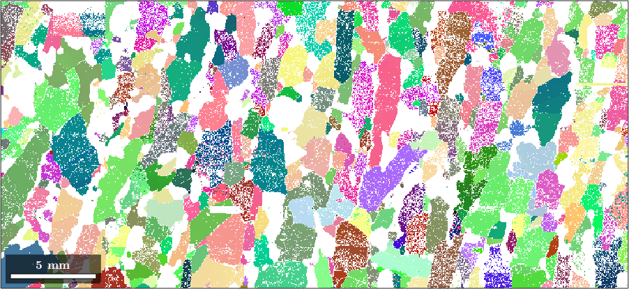

Individual grains appear as flat, well-separated colours. This makes the map look decisive, but it does not reveal where the colour scale wraps. Plotting the key in its default sections also looks deceptively smooth.

plot(colorKey)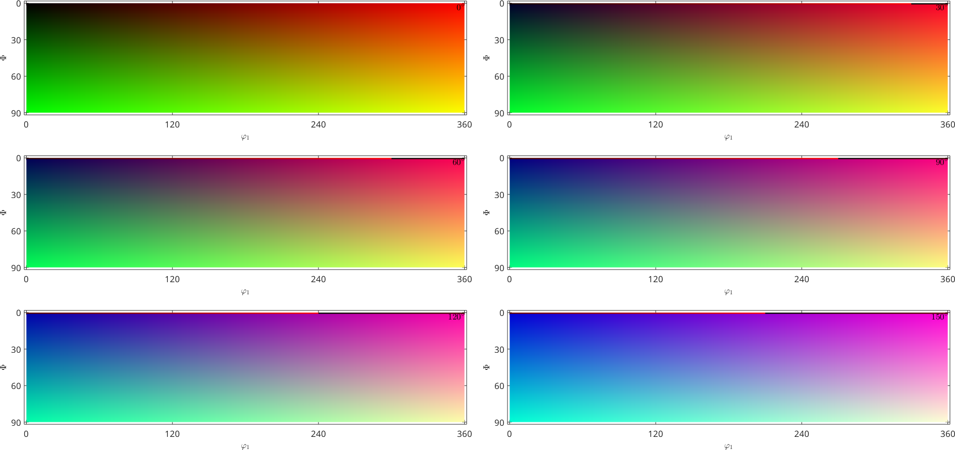

Sigma sections cut orientation space at constant \(\sigma = \varphi_1-\varphi_2\). They expose the seams hidden by the default view.

plot(colorKey,'sections',6,'sigma')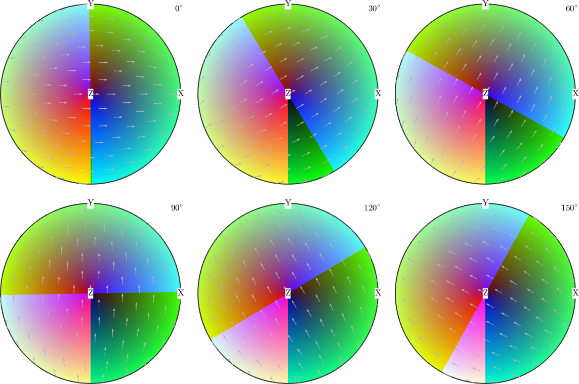

Along several section edges the colour changes abruptly although the orientations remain close. Two nearly identical grains can therefore be drawn in unrelated colours. Treat such a colour edge as a property of the key until another measurement or map confirms a physical boundary.

Marking one orientation

A different question is where the map lies near one chosen orientation. A spotColorKey gives the centre its chosen colour and fades towards white with increasing disorientation.

colorKey = spotColorKey(ebsd('Fo'));
colorKey.center = mean(ebsd('Forsterite').orientations,'robust');
colorKey.color = [0,0,1];
colorKey.psi = SO3DeLaValleePoussinKernel('halfwidth',20*degree);

plot(ebsd('fo'),colorKey.orientation2color(ebsd('fo').orientations))

% plot the corresponding key in orientation space
figure(2)
plot(colorKey,'sections',9,'sigma')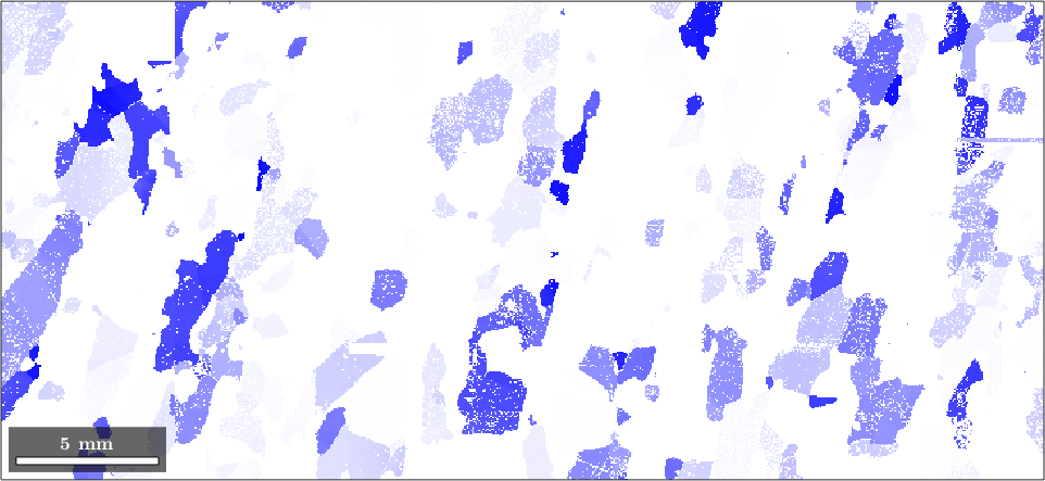

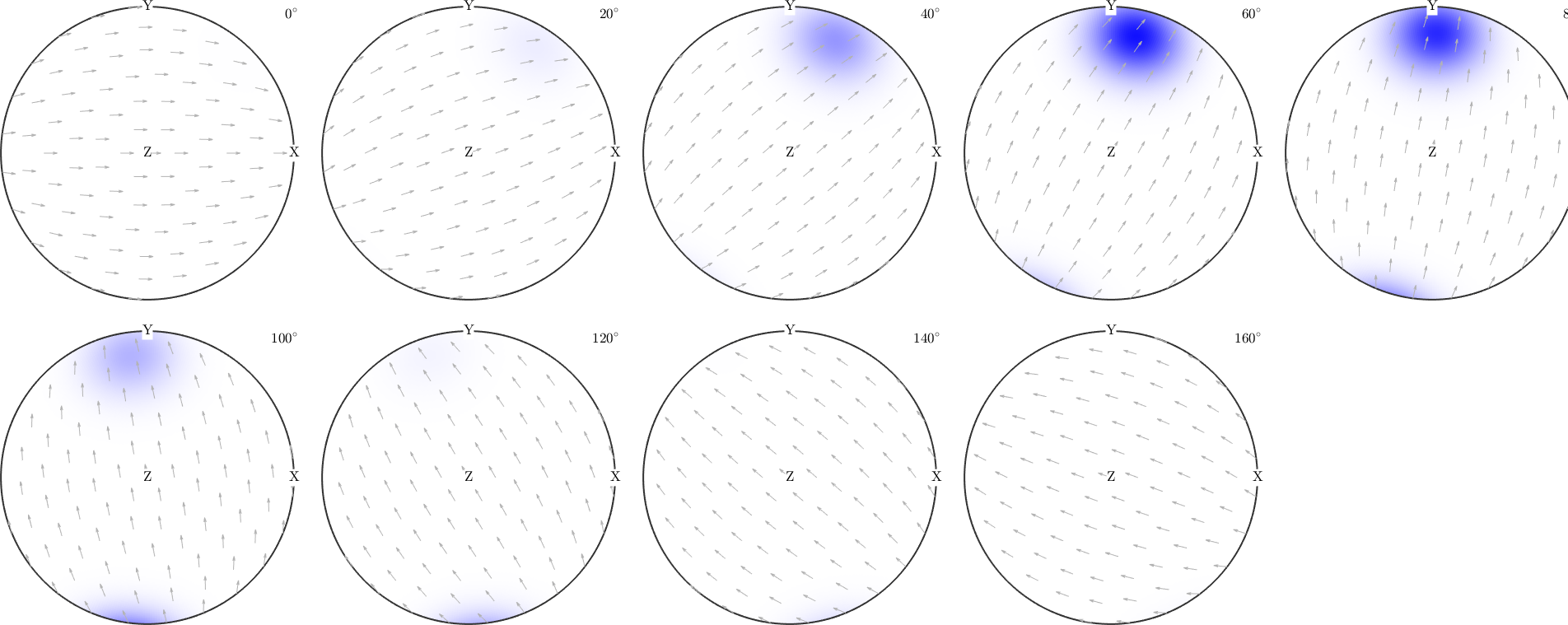
Blue marks orientations near the robust mean, and white marks orientations far from it. The corresponding key shows that this is a three-dimensional neighbourhood in orientation space, not a range on a single Euler angle.

The 20° halfwidth is where the kernel, and hence the blue saturation, falls to half its value at the centre. The fade has no hard edge. To count a specified neighbourhood, use volume with an explicit radius.

spotPercent = 100 * volume(ebsd('fo').orientations,...
  colorKey.center,20*degree)

spotPercent =
   12.1409

12.1% of the indexed forsterite measurements lie within 20° of the robust mean. Because this equally spaced map gives every measurement the same weight, the result is an area-weighted measurement fraction, not a bulk specimen volume fraction.

A density estimate asks a related but different question. It replaces each measurement by a kernel and adds the kernels, so the result depends on the chosen 10° halfwidth.

close all;
odf = calcDensity(ebsd('fo').orientations,'halfwidth',10*degree,'silent');
plot(odf,'sections',9,'silent','sigma')
mtexColorbar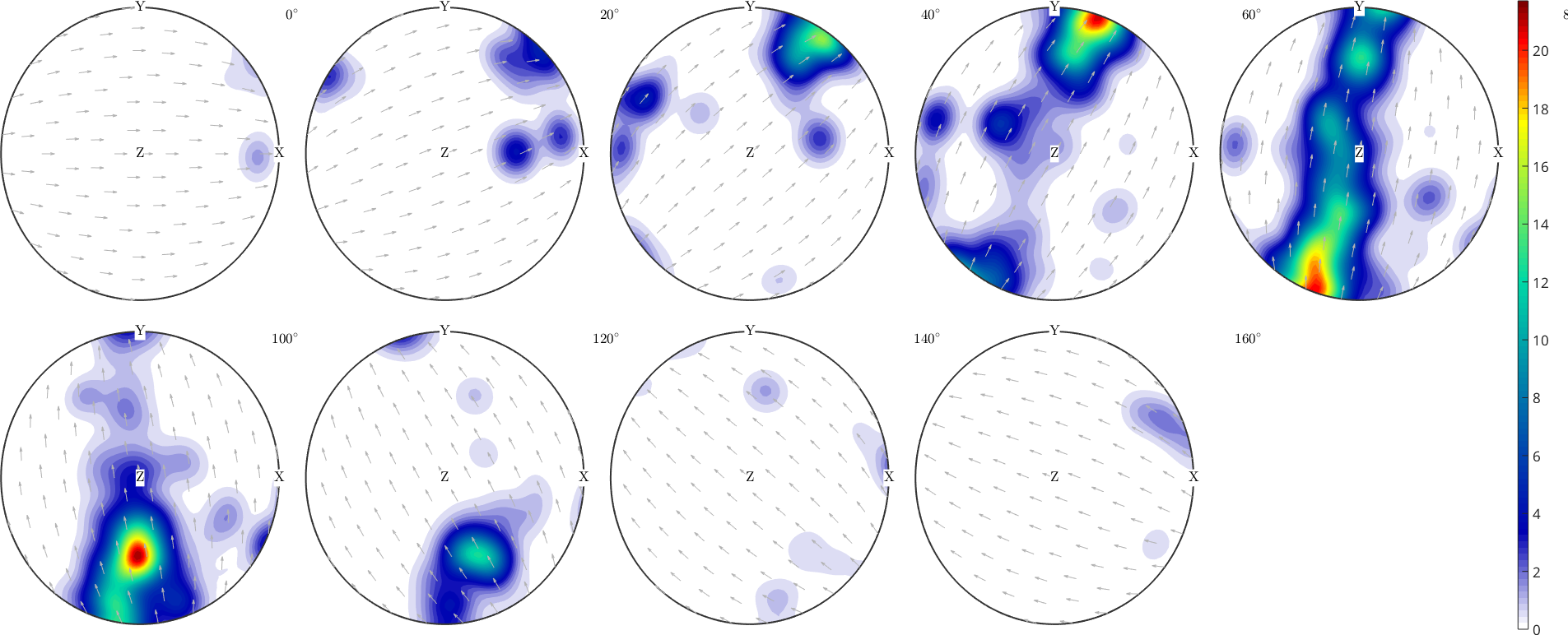

The density plot contains a pronounced maximum in the same part of orientation space as the blue spot. It corroborates the concentration, but its peak height is a density rather than the percentage printed above. ODF Estimation explains the weighting and bandwidth choices.

Marking a fibre

An orientation fibre is the set of all orientations that map one crystal direction h onto one specimen direction r. Rotation about r remains free, so a fibre is a one-dimensional family rather than one orientation.

% define the fibre with the crystal (111) pole parallel to the specimen normal
f = fibre(Miller(1,1,1,csFo),zvector);

% colour directions near the fibre
colorKey = ipfSpotKey(csFo);
colorKey.ipfDirection = f.r;
colorKey.center = f.h;
colorKey.color = [0 0 1];
colorKey.psi = S2DeLaValleePoussinKernel('halfwidth',7.5*degree);

plot(ebsd('fo'),colorKey.orientation2color(ebsd('fo').orientations))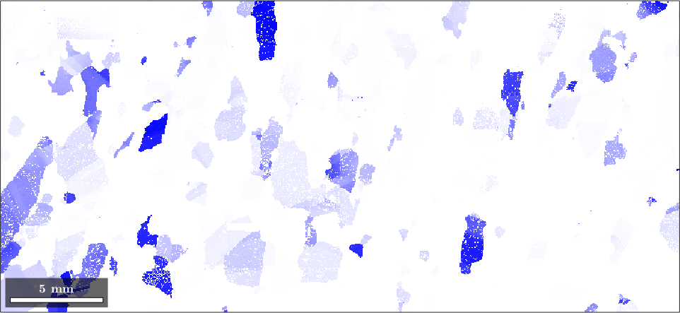

The blue grains have their crystal \((111)\) pole near the specimen normal. This key measures angular distance in the inverse pole figure, so it ignores the free rotation about the normal exactly as the fibre does.

plot(colorKey)

circle(f.h.project2FundamentalRegion,15*degree,'linewidth',2)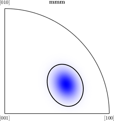

The kernel halfwidth is 7.5°, where the blue saturation has fallen by half. The circle is deliberately larger: it marks the 15° radius used for the hard count below. The colour continues to fade outside the circle.

fibrePercent = 100 * volume(ebsd('fo').orientations,f,15*degree)
hold on
plot(ebsd('fo').orientations,'markercolor','k',...
  'MarkerSize',10,'points',1000,'MarkerAlpha',0.2)
hold off

fibrePercent =
   24.8009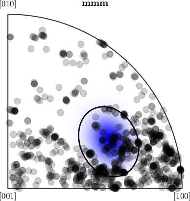

24.8% of the indexed forsterite measurements have their \((111)\) pole within 15° of the specimen normal. The black dots are a random sample of the measured inverse pole figure directions.

The circle covers 13.5% of the fundamental sector, so 24.8% of the measurements inside it is an enrichment of 1.8 times. That enrichment is what the count reports. Smoothed with the same 7.5° kernel the blue centre reaches 1.8 mrd, while the maximum of the sector, 3.4 mrd, lies about 20° away and outside the circle. A fibre count therefore answers how much of the map lies near the chosen direction, and leaves the question of which direction is preferred to a density.

Marking several fibres

Several crystal directions can be highlighted at once. Each centre needs one RGB row in colorKey.color.

% centres in the inverse pole figure
colorKey.center = Miller({0 0 1},{0 1 1},{1 1 1},{11 4 4},{5 0 2},...
  {5 5 2},csFo);

% one colour for each centre
colorKey.color = [[1 0 0];[0 1 0];[0 0 1];[1 0 1];[1 1 0];[0 1 1]];

plot(colorKey)
hold on
plot(ebsd('fo').orientations,'MarkerFaceColor','none',...
  'MarkerEdgeColor','k','MarkerSize',5,'points',5000,'MarkerAlpha',0.2)
hold off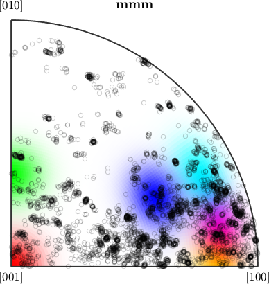

The key contains six coloured lobes, and the black measurements show which lobes the data occupies. This is not a nearest-centre classification. Every centre contributes its fading kernel, so nearby lobes blend where they overlap and orientations far from all centres remain pale.

close all;
plot(ebsd('fo'),colorKey.orientation2color(ebsd('fo').orientations))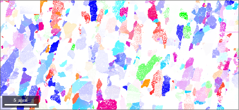

The map now locates six fibre components at once. Compare a pixel with the key to identify the contributing crystal direction; do not read the colour as a complete orientation.

Combining two maps in one figure

A highlighted component is easier to place when the microstructure remains visible underneath it. Draw band contrast first, then add the spot colours with the FaceAlpha option.

close all;
plot(ebsd,ebsd.bc,'micronbar','off')
mtexColorMap black2white

colorKey = ipfSpotKey(csFo);
colorKey.ipfDirection = zvector;
colorKey.center = Miller(1,1,1,csFo);
colorKey.color = [0 0 1];
colorKey.psi = S2DeLaValleePoussinKernel('halfwidth',7.5*degree);

hold on
plot(ebsd('fo'),colorKey.orientation2color(ebsd('fo').orientations),...
  'FaceAlpha',0.5)
hold off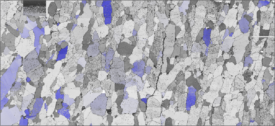

Blue locates the forsterite measurements near the selected fibre. The grey band-contrast layer keeps boundaries and pattern-quality structure visible. Transparency changes only the rendering; it does not change the EBSD data or the angular selection.

Choosing the key

Use a Bunge key only when retaining all three Euler parameters matters, and check its seams before interpreting a colour edge. Use a spot key to locate one orientation and an IPF spot key to locate a fibre. Use volume for a hard angular count and an ODF for a smoothed density estimate.

Small intragranular changes need a reference-based key rather than a global one; Sharp Color Keys develops that case. The following pages turn from display to measurements of local lattice rotation: KAM compares neighbouring pixels, while Mis2Mean / GROD compares each pixel with its grain reference orientation.

Further reading