SO(3)-Kernel Functions

SO(3)-Kernel Functions edit page

Also take a look at the page ODFShapes.

We examine some radial symmetric kernel functions \(\tilde \psi \colon \mathcal{SO}(3) \to \mathbb R\) on \(\mathcal{SO}(3)\). For rotations \({\bf R} \in \mathcal{SO}(3)\) we write this \(\mathcal{SO}(3)\)-kernels as functions of \(t = \cos\frac{\omega ({\bf R})}2\) on the real numbers. Hence we write

\[ \psi(t) = \tilde\psi ({\bf R}). \]

Moreover, we have \(\psi \in L^2([-1,1],\sqrt{1-t^2}\mathrm{d}t)\) and we describe these rotational kernel functions by there Chebyshev expansion

\[ \psi(t) = \sum\limits_{n=0}^{\infty} \hat\psi_n \, \mathcal U_{2n}(t) \]

where \(\mathcal U_{n}\) denotes the Chebyshev polynomials of second kind and degree \(n\in \mathbb N\).

The class SO3Kernel is needed in MTEX to define the specific form of unimodal ODFs. It has to be passed as an argument when calling the methods uniformODF. Furthermore \(\mathcal{SO}(3)\)-Kernels are also used for computing an ODF from EBSD data.

Within the class SO3Kernel kernel functions are represented by their Chebyshev coefficients, that are stored in the field fun.A. As an example lets define an \(\mathcal{SO}(3)\) kernel function with Chebyshev coefficients \(a_0 = 1\), \(a_1 = 0\), \(a_2 = 3\) and \(a_3 = 1\)

psi = SO3Kernel([1;0;3;1])

psi = SO3Kernel
  bandwidth: 3
  halfwidth: 40°

We plot this function by evaluation of its Chebychev series in \(\cos(\frac{\omega}{2})\) for \(\omega \in [-\pi,\pi]\).

plot(psi)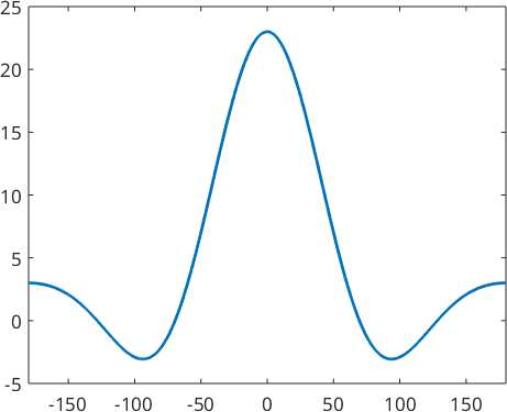

We can define an SO3Fun from a kernel function \(\psi\) at a specific orientation \(\bf R\) by using the class SO3FunRBF, i.e.

psi =SO3DeLaValleePoussinKernel('halfwidth',20*degree)
SO3F = SO3FunRBF(orientation.rand,psi)
plot(SO3F)

psi = SO3DeLaValleePoussinKernel
  bandwidth: 13
  halfwidth: 20°
 
 
SO3F = SO3FunRBF (1 → xyz)
 
  unimodal component
  kernel: de la Vallee Poussin, halfwidth 20°
  center: 1 orientations
 
  Bunge Euler angles in degree
     phi1     Phi    phi2  weight
  156.958 161.468 197.878       1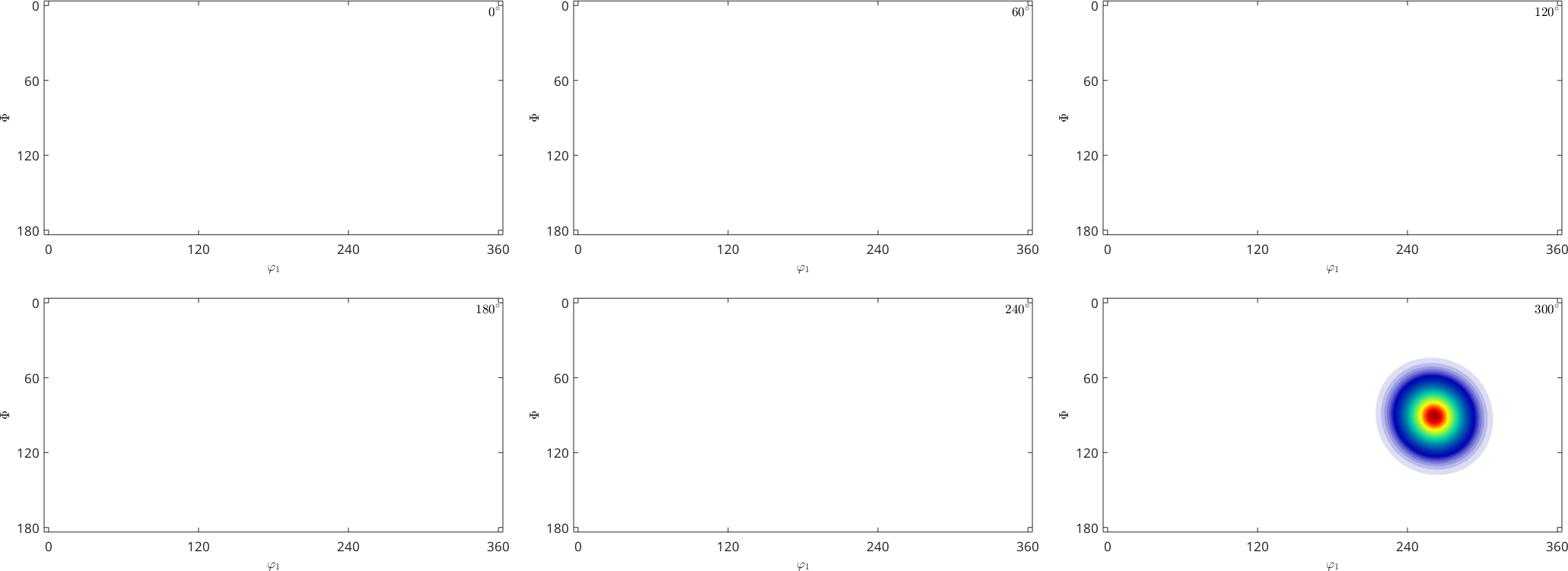

The following kernel function are predefined in MTEX

de la Vallee Poussin kernel (used for ODF, MODF, Pole figures, etc)
Dirichlet kernel (used for physical properties)
Abel Poisson kernel
von Mises Fisher kernel
Gauss Weierstrass kernel
Sobolev kernel
Laplace kernel
Square Singularity kernel
Bump kernel

A specific \(\mathcal{SO}(3)\) kernel function like the de la Vallee Poussin kernel is specified by a half-width angle in orientation space (\(\mathcal{SO}(3)\)) or bandwidth in Fourier space, which is the maximum development in Fourier coefficients.

psi = SO3DeLaValleePoussinKernel('halfwidth',30*degree)

close all
plot(psi)

psi = SO3DeLaValleePoussinKernel
  bandwidth: 9
  halfwidth: 30°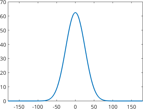

In the following we want to look at some different types of \(\mathcal{SO}(3)\) kernel functions.

The de La Vallee Poussin Kernel

The de la Vallee Poussin kernel on \(\mathcal{SO}(3)\) is defined by

\[ K(t) = \frac{B(\frac32,\frac12)}{B(\frac32,\kappa+\frac12)}\,t^{2\kappa}\]

for \(t\in[0,1]\), where \(B\) denotes the Beta function. The de la Vallee Poussin kernel additionaly has the unique property that for a given halfwidth it can be described exactly by a finite number of Fourier coefficients. This kernel is recommended for Texture analysis as it is always positive in orientation space and there is no truncation error in Fourier space. Hence we can define the de la Vallee Poussin kernel \(\psi_{\kappa}\) depending on a parameter \(\kappa \in \mathbb N \setminus \{0\}\) by its finite Chebyshev expansion

\[ \psi_{\kappa}(t) = \frac{(\kappa+1)\,2^{2\kappa-1}}{\binom{2\kappa-1}{\kappa}} \, t^{2\kappa} = \binom{2\kappa+1}{\kappa}^{-1} \, \sum\limits_{n=0}^{\kappa} (2n+1)\,\binom{2\kappa+1}{\kappa-n} \, \mathcal U_{2n}(t).\]

Lets construct two of them.

psi1 = SO3DeLaValleePoussinKernel('halfwidth',15*degree)
psi2 = SO3DeLaValleePoussinKernel('halfwidth',20*degree)

plot(psi1)
hold on
plot(psi2)
hold off
legend('halfwidth = 15°','halfwidth = 20°')

psi1 = SO3DeLaValleePoussinKernel
  bandwidth: 17
  halfwidth: 15°
 
 
psi2 = SO3DeLaValleePoussinKernel
  bandwidth: 13
  halfwidth: 20°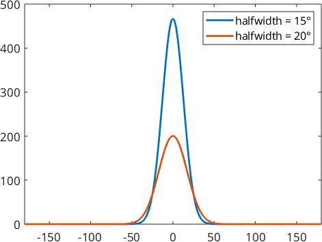

Here the parameter \(\kappa\) is \(40.34\) for function \(\psi_1\) and \(22.64\) in function \(\psi_2\).

We also take a look at the Fourier coefficients

plotSpektra(psi1)
hold on
plotSpektra(psi2)
hold off
legend('halfwidth = 15°','halfwidth = 20°')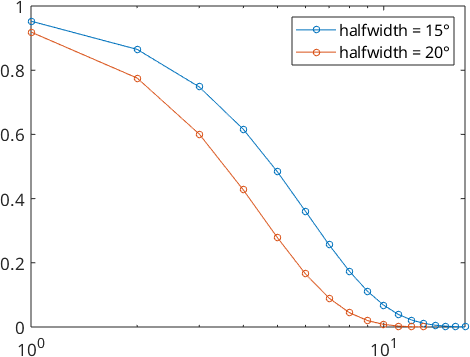

The Dirichlet Kernel

The Dirichlet kernel has the unique property of being a convergent finite series in Fourier coefficients with an integral of one. This kernel is recommended for calculating physical properties as the Fourier coefficients always have a value of one for a given bandwidth.

On the rotation group \(\mathcal{SO}(3)\) the Dirichlet kernel \(\psi_N \in L^2(\mathcal{SO}(3))\) is defined by its Chebyshev series

\[ \psi_N(t) = \sum\limits_{n=0}^N (2n+1) \, \mathcal U_{2n}(t).\]

Lets construct two of them.

psi1 = SO3DirichletKernel(10)
psi2 = SO3DirichletKernel(5)

plot(psi1)
hold on
plot(psi2)
hold off
legend('bandwidth = 5','bandwidth = 10')

psi1 = SO3DirichletKernel
  bandwidth: 10
  halfwidth: 13°
 
 
psi2 = SO3DirichletKernel
  bandwidth: 5
  halfwidth: 24°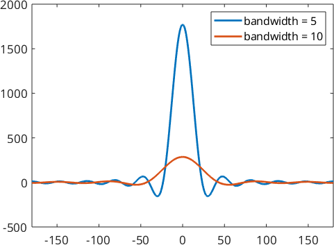

By looking at the fourier coefficients we see, that they are exactly 1.

plotSpektra(psi1)
hold on
plotSpektra(psi2)
hold off
legend('bandwidth = 5','bandwidth = 10')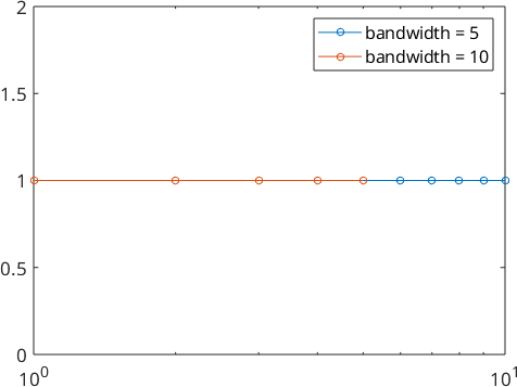

The Abel Poisson Kernel

The Abel Poisson kernel \(\psi_{\kappa}\in L^2(\mathcal{SO}(3))\) is a nonnegative function depending on a parameter \(\kappa \in (0,1)\) and is defined by its Chebyshev series

\[ \psi_{\kappa}(t) = \sum\limits_{n=0}^{\infty} (2n+1) \, \kappa^{2n} \, \mathcal U_{2n}(t).\]

Lets construct two of them.

psi1 = SO3AbelPoissonKernel('halfwidth',15*degree)
psi2 = SO3AbelPoissonKernel('halfwidth',20*degree)

plot(psi1)
hold on
plot(psi2)
hold off
legend('halfwidth = 15°','halfwidth = 20°')

psi1 = SO3AbelPoissonKernel
  bandwidth: 19
  halfwidth: 15°
 
 
psi2 = SO3AbelPoissonKernel
  bandwidth: 15
  halfwidth: 20°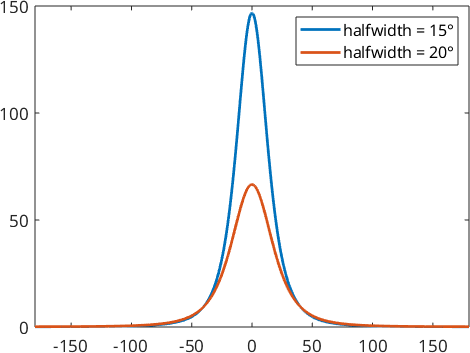

Here the parameter \(\kappa\) is \(0.82\) for function \(\psi_1\) and \(0.76\) in function \(\psi_2\).

We also take a look at the Fourier coefficients

plotSpektra(psi1)
hold on
plotSpektra(psi2)
hold off
legend('halfwidth = 15°','halfwidth = 20°')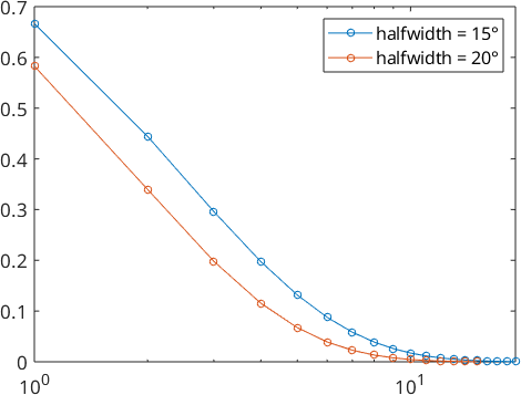

The von Mises Fisher Kernel

The von Mises Fisher kernel \(\psi_{\kappa}\in L^2(\mathcal{SO}(3))\) is a nonnegative function depending on a parameter \(\kappa>0\) and is defined by its Chebyshev series

\[ \psi_{\kappa}(t) = \sum_{n=0}^{\infty} \frac{\mathcal{I}_n(\kappa)-\mathcal{I}_{n+1}(\kappa)}{\mathcal{I}_0(\kappa)-\mathcal{I}_1(\kappa)} \, \mathcal U_{2n}(t)\]

or directly by

\[ \psi_{\kappa}(\cos\frac{\omega({\bf R})}2) = \frac1{\mathcal{I}_0(\kappa)-\mathcal{I}_1(\kappa)} \, \mathrm{e}^{\kappa \cos\omega({\bf R})}\]

while \(\mathcal I_n,\,n \in \mathbb N_0\) denotes the the modified Bessel functions of first kind

\[ \mathcal I_n (\kappa) = \frac1{\pi} \int_0^{\pi} \mathrm e^{\kappa \, \cos \omega} \, \cos n\omega \, \mathrm d\omega. \]

Lets construct two of this kernels.

psi1 = SO3vonMisesFisherKernel('halfwidth',15*degree)
psi2 = SO3vonMisesFisherKernel('halfwidth',20*degree)

plot(psi1)
hold on
plot(psi2)
hold off
legend('halfwidth = 15°','halfwidth = 20°')

psi1 = SO3vonMisesFisherKernel
  bandwidth: 18
  halfwidth: 15°
 
 
psi2 = SO3vonMisesFisherKernel
  bandwidth: 14
  halfwidth: 20°

Here the parameter \(\kappa\) is \(20.34\) for function \(\psi_1\) and \(11.49\) in function \(\psi_2\).

We also take a look at the Fourier coefficients

plotSpektra(psi1)
hold on
plotSpektra(psi2)
hold off
legend('halfwidth = 15°','halfwidth = 20°')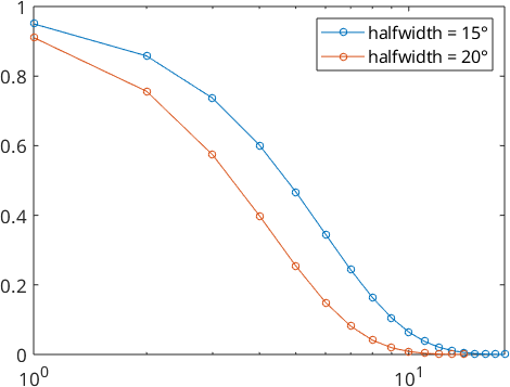

The Gauss Weierstrass Kernel

The Gauss Weierstrass kernel \(\psi_{\kappa}\in L^2(\mathcal{SO}(3))\) is a nonnegative function depending on a parameter \(\kappa>0\) and is defined by its Chebyshev series

\[ \psi_{\kappa}(t) = \sum\limits_{n=0}^{\infty} (2n+1) \, \mathrm e^{-n(n+1)\kappa} \, \mathcal U_{2n}(t).\]

Lets construct two of them by the parameter \(\kappa\).

psi1 = SO3GaussWeierstrassKernel(0.025)
psi2 = SO3GaussWeierstrassKernel(0.045)

plot(psi1)
hold on
plot(psi2)
hold off
legend('halfwidth = 15°','halfwidth = 20°')

psi1 = SO3GaussWeierstrassKernel
  bandwidth: 17
  halfwidth: 15°
 
 
psi2 = SO3GaussWeierstrassKernel
  bandwidth: 13
  halfwidth: 20°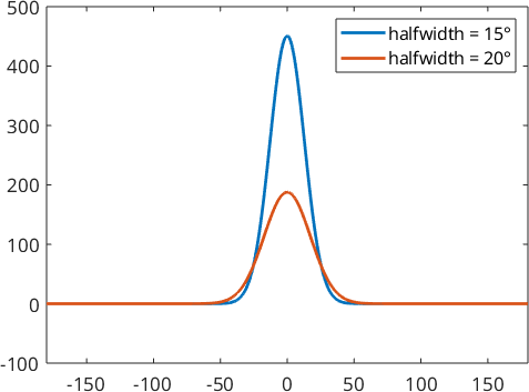

We also take a look at the Fourier coefficients

plotSpektra(psi1)
hold on
plotSpektra(psi2)
hold off
legend('halfwidth = 15°','halfwidth = 20°')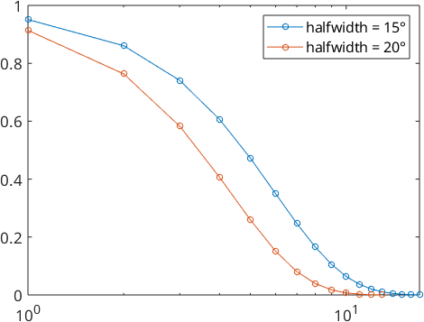

The Sobolev Kernel

The Sobolev kernel \(\psi_{s}\in L^2(\mathcal{SO}(3))\) is a radial symmetric kernel function depending on a parameter \(s\) and is defined by its Chebyshev series

\[ \psi_s(t) = \sum\limits_{n=0}^{\infty} (2n+1)\, (n(n+1))^s \, \mathcal U_{2n}(t). \]

Lets construct two of them by the parameter \(s\) and banwidth 15.

psi1 = SO3SobolevKernel(1,'bandwidth',15)
psi2 = SO3SobolevKernel(1.2,'bandwidth',15)

plot(psi1)
hold on
plot(psi2)
hold off
legend('s = 1','s = 1.2')

psi1 = SO3SobolevKernel
  bandwidth: 15
  halfwidth: 8.1°
 
 
psi2 = SO3SobolevKernel
  bandwidth: 15
  halfwidth: 8°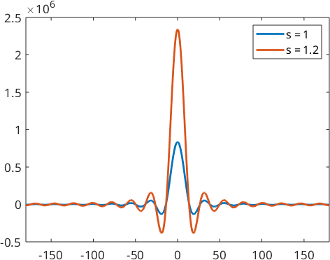

We also take a look at the Fourier coefficients

plotSpektra(psi1)
hold on
plotSpektra(psi2)
hold off
legend('s = 1','s = 1.2')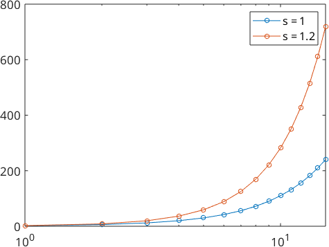

The Laplace Kernel

The Laplace kernel \(\psi\in L^2(\mathcal{SO}(3))\) is a radial symmetric kernel function which is defined by its Chebyshev series

\[ \psi(t) = \sum\limits_{n=0}^{\infty} \frac{(2n+1)}{4\,n^2\,(2n+2)^2} \, \mathcal U_{2n}(t). \]

psi = SO3LaplaceKernel

plot(psi)

psi = SO3LaplaceKernel
  bandwidth: 4
  halfwidth: 55°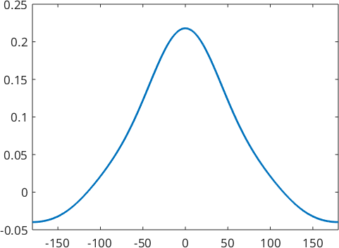

We also take a look at the Fourier coefficients

plotSpektra(psi)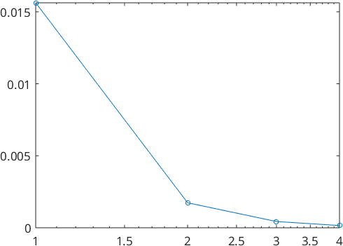

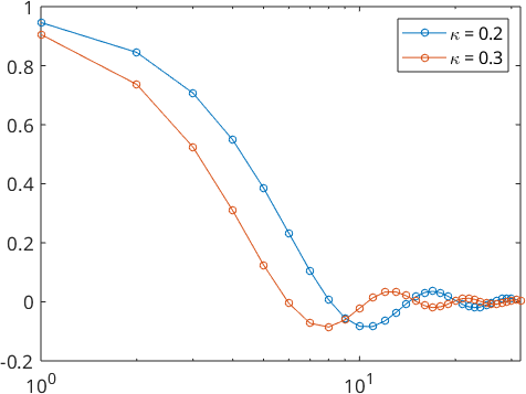
The Squared Singularity Kernel

The squared singularity kernel \(\psi_{\kappa}\in L^2(\mathcal{SO}(3))\) is a nonnegative function depending on a parameter \(\kappa\in(0,1)\) and is defined by its Chebyshev series

\[ \psi_{\kappa}(t) = \sum\limits_{n=0}^{\infty} \hat{f}_n(\kappa) \, \mathcal U_{2n}(t). \]

where the chebychev coefficients follows a 3-term recurrsion

\(\hat{f}_0 = 1\)

\(\hat{f}_1 = \frac{1+\kappa^2}{2\kappa}-\frac1{\log\frac{1+\kappa}{1-\kappa}}\)

\(\hat{f}_n = \frac{(2n-3)(2n+1)(1+\kappa^2)}{(2n-1)(n-1)2\kappa} \, \hat{f}_{n-1}(\kappa)-\frac{2\kappa(n-2)(2n+1)}{2n-3} \, \hat{f}_{n-2}(\kappa)\).

Lets construct two of them by the parameter \(\kappa\).

psi1 = SO3SquareSingularityKernel(0.2)
psi2 = SO3SquareSingularityKernel(0.3)

plot(psi1)
hold on
plot(psi2)
hold off
legend('\kappa = 0.2','\kappa = 0.3')

psi1 = SO3SquareSingularityKernel
  bandwidth: 5
  halfwidth: 78°
 
 
psi2 = SO3SquareSingularityKernel
  bandwidth: 7
  halfwidth: 55°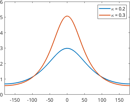

We also take a look at the Fourier coefficients

plotSpektra(psi1)
hold on
plotSpektra(psi2)
hold off
legend('\kappa = 0.2','\kappa = 0.3')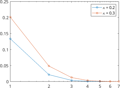

The Bump kernel

The bump kernel \(\tilde\psi_r\in L^2(\mathcal{SO}(3))\) is a radial symmetric kernel function depending on a parameter \(r\in (0,\pi)\). The function value is 0, if the angle is greater then the halfwidth \(r\). Otherwise it is has a contstant value, such that the mean of \(\psi_r\) on \(\mathcal{SO}(3)\) is 1. Hence we use the open set

\[U_r = \{ {\bf R} \in \mathcal{SO}(3) \,\vert ~ \lvert \omega( {\bf R})\rvert <r \}\]

and define the bump kernel by

\[ \tilde\psi_r( {\bf R}) = \frac1{\lvert U_r \rvert } \mathbf{1}_{ \{ {\bf R} \in U_r \} } \]

where \(\mathbf{1}\) is the indicator function.

The main problem of the bump kernel is that we need a lot of chebychev coefficients to describe it. That possibly can result in high runtimes.

psi1 = SO3BumpKernel(30*degree)
psi2 = SO3BumpKernel(40*degree)

plot(psi1)
hold on
plot(psi2)
hold off
legend('halfwidth = 30°','halwidth = 40°')

psi1 = SO3BumpKernel
  bandwidth: 1000
  halfwidth: 30°
 
 
psi2 = SO3BumpKernel
  bandwidth: 1000
  halfwidth: 40°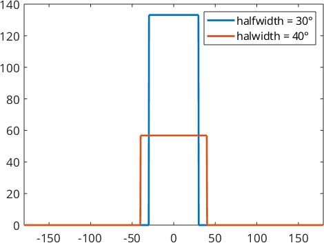

We also take a look at the Fourier coefficients

plotSpektra(psi1)
hold on
plotSpektra(psi2)
hold off
legend('\kappa = 0.2','\kappa = 0.3')