Misorientation Distribution Function

A single misorientation describes one pair of crystals. A map contains thousands of such pairs. Their density in misorientation space is the misorientation distribution function, or MDF.

There are two MDFs, and confusing them changes the physical question:

The uncorrelated MDF is what the two textures alone imply. It is not a uniform distribution unless both textures are uniform. The boundary MDF also contains the effect of which orientations became neighbours. Comparing the two separates a preferred orientation relationship from an accidental consequence of texture.

This page assumes familiarity with misorientation theory, grain reconstruction, and kernel density estimation. The plotting frame below matches the specimen frame stored with this data set.

plottingConvention.default('y↑→x');
mtexdata forsterite silent

grains = calcGrains(ebsd);

The Boundary Misorientation Distribution Function

First take the misorientation of every forsterite--enstatite boundary segment. The displayed summary identifies the mapping from the forsterite crystal frame to the enstatite crystal frame and reports 11,751 samples.

mori_boundary = grains.boundary('Fo','En').misorientation

mori_boundary = misorientation (Forsterite → Enstatite)
  size: 11751 × 1

This is one sample per boundary segment, not one vote per neighbouring grain pair. A long boundary therefore contributes more samples than a short one. The result also depends on how finely the boundary was sampled.

calcDensity estimates the density, just as it does for a list of orientations. The halfwidth is the angular smoothing scale. A smaller value resolves sharper peaks but also more sampling noise.

mdf_boundary = calcDensity(mori_boundary,'halfwidth',5*degree)

mdf_boundary = SO3FunHarmonic (Forsterite → Enstatite)
  bandwidth: 48
  weight: 1

The result is an SO(3) function and supports everything such a function does. MTEX normalizes its mean density to one, so values are commonly read as multiples of a random distribution (mrd). Its maximum gives the preferred misorientation.

[peakMRD,preferredMori] = max(mdf_boundary);

peakMRD

peakMRD =
  118.3380

preferredAxis = round(axis(preferredMori))

preferredAxis = Miller (222)
  h k l
  0 0 1

preferredAngle = angle(preferredMori) ./ degree

preferredAngle =
   89.9817

The peak is 118.34 mrd at \(89.98^\circ\) about \((001)\) in the forsterite crystal frame. Forsterite and enstatite share lattice planes in this relationship, and it dominates the phase boundaries of this map.

An axis--angle section at \(90^\circ\) cuts through this maximum.

plotSection(mdf_boundary,'axisAngle',90*degree)
mtexColorbar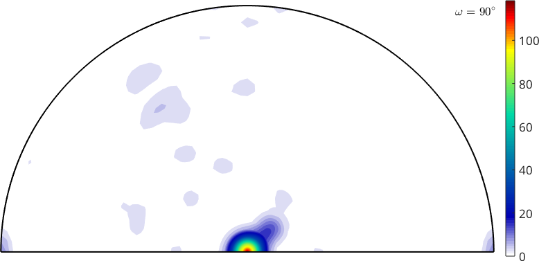

The narrow red spot at the middle of the lower edge is the \((001)\) peak. Most other axes in this section have density close to zero.

The Uncorrelated Misorientation Distribution Function

calcMisorientation draws random pairs of EBSD pixels without requiring them to be neighbours. By default it draws 100,000 pairs and rejects points closer than one percent of the map diagonal. Fixing the random seed makes the published example reproducible.

rng default;
mori_uncorrelated = calcMisorientation(ebsd('En'),ebsd('Fo'))

mori_uncorrelated = misorientation (Forsterite → Enstatite)
  size: 99978 × 1

The summary reports 99,978 accepted pairs. These are pixel orientations, not grain mean orientations, so large phases and densely sampled regions contribute more strongly than small ones.

mdf_uncorrelated = calcDensity(mori_uncorrelated)

mdf_uncorrelated = SO3FunHarmonic (Forsterite → Enstatite)
  bandwidth: 25
  weight: 1

uncorrelatedPeakMRD = max(mdf_uncorrelated)

uncorrelatedPeakMRD =
    2.0566

Its maximum is 2.06 mrd, not 118.34 mrd. The preferred boundary relationship is absent from independently paired pixels. The boundary peak is therefore a property of the boundary network, not something the two textures produce by themselves.

plotSection(mdf_uncorrelated,'axisAngle',90*degree)
mtexColorbar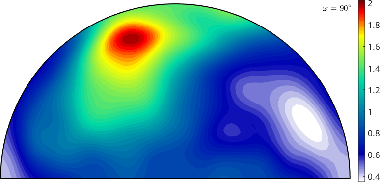

The maximum is now a broad lobe rather than the narrow \((001)\) spot. The colorbar also shows that its scale is about two orders of magnitude lower.

The Uncorrelated MDF from Two ODFs

The uncorrelated MDF needs no individual orientations at all. It is completely determined by the two orientation distribution functions (ODFs). The ODFs below use the same pixel weighting as the direct sample.

odf_fo = calcDensity(ebsd('fo').orientations,'halfwidth',10*degree);
odf_en = calcDensity(ebsd('en').orientations,'halfwidth',10*degree);

calcMDF computes their convolution. The argument order below gives the same forsterite-to-enstatite mapping as the boundary misorientations.

mdf_from_odfs = calcMDF(odf_en,odf_fo)

mdf_from_odfs = SO3FunHarmonic (Forsterite → Enstatite)
  bandwidth: 25
  weight: 1

This and the direct estimate describe the same uncorrelated population. Their relative difference is

relativeDifferencePercent = 100 * ...
  norm(mdf_from_odfs - mdf_uncorrelated) ./ norm(mdf_uncorrelated)

relativeDifferencePercent =
    4.9397

The difference is 4.94 percent in the \(L^2\) norm. The ODF route smooths each texture before convolution, whereas the direct route smooths the sampled pair differences once. Finite random sampling contributes as well; the difference does not indicate different physical content.

plotSection(mdf_from_odfs,'axisAngle',90*degree)
mtexColorbar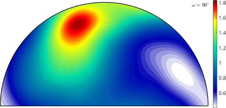

The broad maximum and the low-density patch on the right match the direct estimate above. The agreement is visible in both location and scale.

With one ODF, calcMDF gives the uncorrelated misorientations within one phase. The displayed antipodal: true records that a same-phase pair has grain exchange symmetry.

mdf_fo = calcMDF(odf_fo)

mdf_fo = SO3FunHarmonic (Forsterite → Forsterite)
  antipodal: true
  bandwidth: 25
  weight: 1

Angle Distribution

An MDF is a function on a three-dimensional space. Integrating out the misorientation axis leaves the one-dimensional angle distribution.

close all
plotAngleDistribution(mori_boundary,'figSize','small')
hold on
plotAngleDistribution(mdf_from_odfs)
hold off
legend('boundary','uncorrelated')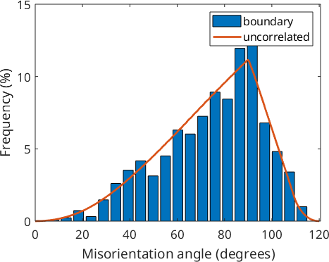

The boundary histogram has an extra peak near \(90^\circ\). The uncorrelated curve has no matching spike, although it follows the broader trend of the histogram. An angle peak alone does not identify the complete orientation relationship because the axis has been integrated out.

Uniform orientations provide a third reference. Their angle distribution is not flat: large rotation angles occupy more of rotation space than small ones, and crystal symmetry limits the largest distinct angle. This geometry is illustrated in Plotting Rotations.

close all
plotAngleDistribution(mdf_from_odfs,'figSize','small')
hold on
plotAngleDistribution(ebsd('fo').CS,ebsd('en').CS)
hold off
legend('uncorrelated texture','uniform orientations','Location','best')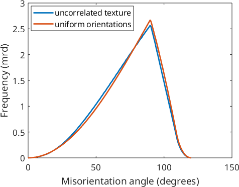

The orange curve is the texture-free baseline, not a horizontal line. The numbers behind the curves come from calcAngleDistribution(mdf) and calcAngleDistribution(ori). See Angle Distribution for their use.

Axis Distribution

The other marginal integrates out the angle and retains the misorientation axis. First consider the boundary misorientations.

plotAxisDistribution(mori_boundary,'smooth')
mtexColorbar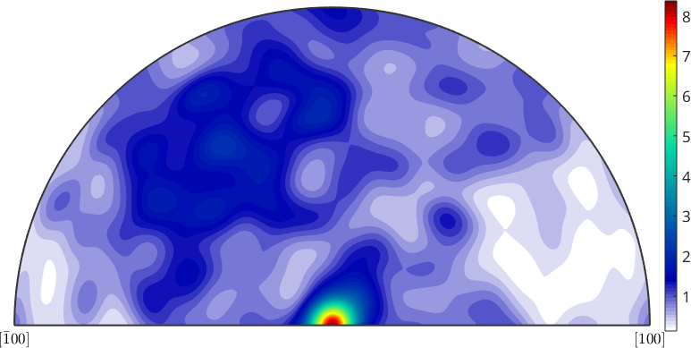

Their axes form a narrow maximum at \((001)\), consistent with the full MDF. The uncorrelated MDF gives a much broader distribution.

plotAxisDistribution(mdf_from_odfs)
mtexColorbar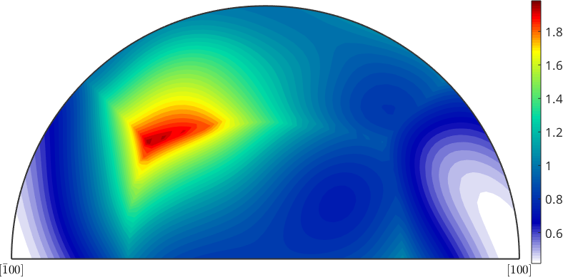

The broad lobe covers much of the symmetry sector rather than collapsing onto the boundary relationship. The marginal is itself a spherical function, returned by calcAxisDistribution.

axisDistribution = calcAxisDistribution(mdf_boundary)

axisDistribution = S2FunHarmonicSym (222)
  bandwidth: 64

References

Next

Continue with Axis Distribution and Angle Distribution for the two marginals and their symmetry-dependent baselines. Theory develops the underlying misorientation, while Twinning applies a preferred misorientation to individual boundaries.