ODFs are functions on the rotation group \(SO(3)\). Therefore we construct them by the class SO3Fun.
MTEX provides a very simple way to define model ODFs. Generally, there are five different ODF types in MTEX:
The central idea is that MTEX allows you to calculate mixture models, by adding and subtracting arbitrary ODFs. Model ODFs may be used as references for ODFs estimated from pole figure data or EBSD data and are instrumental for simulating texture evolution.
The Uniform ODF
The most simplest case of a model ODF is the uniform ODF
\[f(g) = 1,\quad g \in SO(3),\]
which is everywhere identical to one. In order to define a uniform ODF one needs only to specify its crystal and specimen symmetry and to use the command uniformODF.
cs = crystalSymmetry('cubic');
ss = specimenSymmetry('orthorhombic');
odf = uniformODF(cs,ss)
odf = SO3FunRBF (m3̅m → y↑→x (mmm))
uniform component
weight: 1Combining model ODFs
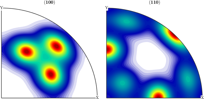
All the above can be arbitrarily rotated and combined. For instance, the classical Santa Fe example can be defined by commands
cs = crystalSymmetry('cubic');
ss = specimenSymmetry('orthorhombic');

psi = SO3vonMisesFisherKernel('halfwidth',10*degree);
mod1 = orientation.byMiller([1,2,2],[2,2,1],cs,ss);

odf =  0.73 * uniformODF(cs,ss) + 0.27 * unimodalODF(mod1,psi)

close all
plotPDF(odf,[Miller(1,0,0,cs),Miller(1,1,0,cs)],'antipodal')
odf = SO3FunRBF (m3̅m → y↑→x (mmm))
uniform component
weight: 0.73
unimodal component
kernel: van Mises Fisher, halfwidth 10°
center: 1 orientations
Bunge Euler angles in degree
phi1 Phi phi2 weight
116.565 48.1897 26.5651 0.27