The Spherical Radon Transform

The spherical Radon transform replaces every function value by an average around a great circle. It therefore turns a localized peak into a ring. This geometric change is the key to recognizing the transform in a plot.

In texture analysis, the corresponding operation turns an ODF into a pole figure. This page first develops the transform for an ordinary spherical function. See calcPDF for the orientation-space version.

From a peak to a ring

Start with a smooth peak centred on the direction \((1,1,1)\).

f = @(v) exp(-4 * angle(v,vector3d(1,1,1)).^2);

sF = S2FunHarmonic.quadrature(f,'bandwidth',48)

sF = S2FunHarmonic (y↓→x)
  bandwidth: 48

plot(sF,'upper')
mtexColorbar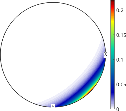

The warm colours are confined to one neighbourhood on the upper hemisphere. This localized maximum is the feature to follow through the transform.

Compute the spherical Radon transform with radon.

rF = radon(sF)

rF = S2FunHarmonic (y↓→x)
  bandwidth: 48
  antipodal: true

plot(rF,'upper')
mtexColorbar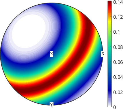

The single maximum has become a ring. Every pole on that ring identifies a great circle that passes through the original peak. Such poles lie \(90\) degree from the peak direction.

Checking one transformed value

Let \(\vec x\) be the pole of a great circle. The transform at \(\vec x\) is the mean of the function along the circle perpendicular to \(\vec x\),

\[ \mathcal R f(\vec x) = \frac{1}{2\pi}\int_{\vec v \perp \vec x} f(\vec v)\,\mathrm{d}\vec v. \]

Check this definition at an arbitrary direction. The vectors u1 and u2 span the plane perpendicular to x, while v samples its unit circle.

x = normalize(vector3d(0.3,-0.7,0.5));

u1 = orth(x); u2 = cross(x,u1);
t = 2*pi*(0:1e5-1).'/1e5;
v = cos(t) .* u1 + sin(t) .* u2;

[mean(sF.eval(v)), rF.eval(x)]

ans =
    0.1389    0.1389

The direct mean and the value returned by radon agree to the displayed precision. The spherical transform is the analogue of the classical Radon transform used in computed tomography.

What information is lost

A great circle contains every direction together with its antipode. Averaging along that circle cannot distinguish \(f(\vec v)\) from \(f(-\vec v)\). The great-circle Radon transform therefore destroys the odd part of a function and is always antipodally symmetric.

Apply the transform to the purely odd function \(f(\vec v)=v_z\). The result is zero up to numerical noise.

sFodd = S2FunHarmonic.quadrature(@(v) v.z,'bandwidth',8);

max(abs(radon(sFodd)))

ans =
   4.8646e-12

Mean values along small circles

A second argument \(\delta\) asks radon to average along a small circle. Its angular distance from \(\vec x\) is \(\pi/2+\delta\), instead of \(\pi/2\) for a great circle.

delta = 20*degree;

rD = radon(sF,delta);

w = cos(pi/2+delta) * x + sin(pi/2+delta) * ...
  (cos(t) .* u1 + sin(t) .* u2);

[mean(sF.eval(w)), rD.eval(x)]

ans =
    0.0727    0.0727

Again, the sampled mean and the transformed value agree to the displayed precision.

plot(rD,'upper')
mtexColorbar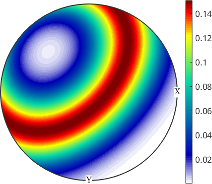

The high-value band is displaced from the great-circle ring because the sampled circles are now offset by delta. For nonzero delta, opposite poles generally describe different small circles, so rD need not be antipodally symmetric.

Inverting the transform

invRadon reverses the transform in the spherical harmonic basis. A round trip recovers an antipodally symmetric function exactly within its harmonic representation, up to floating-point error.

sFeven = S2FunHarmonic.quadrature(@(v) 0.5*(f(v) + f(-v)), ...
  'bandwidth',48);

nodes = equispacedS2Grid('resolution',5*degree);

mean(abs(invRadon(radon(sFeven)).eval(nodes) - sFeven.eval(nodes)))

ans =
   2.9619e-12

A general function cannot be recovered because its odd part has already been lost. Inverting rF returns precisely the even part of sF.

backF = invRadon(rF)

mean(abs(backF.eval(nodes) - sF.eval(nodes)))

backF = S2FunHarmonic (y↓→x)
  bandwidth: 48
  antipodal: true
 
ans =
    0.0599

The nonzero first error measures the missing odd part. Comparing with sFeven instead confirms that the even part was recovered.

mean(abs(backF.eval(nodes) - sFeven.eval(nodes)))

ans =
   3.7083e-12

The maths behind this

Great-circle averaging is unchanged by rotation. The spherical Radon transform is therefore a convolution and acts diagonally on the harmonic expansion. Its Legendre coefficients are

\[ A_n = (-1)^{n/2}\,\frac{(n-1)!!}{n!!} \quad\text{for even } n, \qquad A_n = 0 \quad\text{for odd } n. \]

The zero odd coefficients explain the permanent loss demonstrated above. For the even degrees, invRadon divides by \(A_n\).

The magnitude of \(A_n\) decays like \(n^{-1/2}\). Its inverse consequently amplifies high-degree noise. Measured data should not be inverted directly; instead, solve a regularized problem as in ODF reconstruction from pole figures. The missing odd part reappears there as the ghost effect.

References

Next

Spherical Vector Fields moves from scalar values on the sphere to vectors and shows how to visualize their direction and magnitude.

References

- J. D. McEwen and M. A. Price, Scale-discretised ridgelet transform on the sphere, 27th European Signal Processing Conference (2019), 1-5, derives the convolution and harmonic representations and the exact inverse for antipodally symmetric functions.