A fibre in orientation space is essentially a line connecting two orientations and can be represented in MTEX by a single variable of type fibre. To illustrate the definition of a fibre we first define cube and goss orientation
% define crystal and specimen symmetry
cs = crystalSymmetry('432');
ss = specimenSymmetry('1');

% and two orientations
ori1 = orientation.cube(cs,ss);
ori2 = orientation.goss(cs,ss);
and then the fibre connecting both orientations
f = fibre(ori1,ori2)f = fibre (432 → y↑→x)
h || r: (100) || (1,0,0)
o1 → o2: (0°,0°,0°) → (0°,45°,0°)Finally we plot everything into the Euler space
% plot the fibre
plot(f,'DisplayName','Fibre','linewidth',4,'linecolor','green')

% and on top of it the orientations
hold on
plot(ori1,'DisplayName','CUBE','MarkerSize',12,'MarkerFaceColor','darkred','MarkerEdgeColor','k')
plot(ori2,'DisplayName','GOSS','MarkerSize',12,'MarkerFaceColor','blue','MarkerEdgeColor','k')
hold off
legend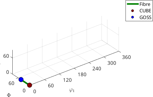
Alternatively, we may visualize the fibre also in axis angle space
% plot the fibre
plot(f,'linecolor','green','linewidth',6,'axisAngle')

% and on top of it the orientations
hold on
plot(ori1,'MarkerFaceColor','darkred','MarkerSize',15,'axisAngle')
plot(ori2,'MarkerFaceColor','blue','MarkerSize',15)
hold off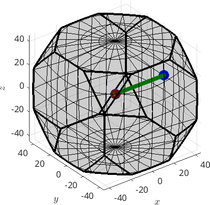
Obviously, f is not a full fibre. Since, the orientation space has no boundary a full fibre is best thought of as a circle that passes trough two fixed orientations. In order to define the full fibre us the option 'full'
f = fibre(ori1,ori2,'full')

hold on
plot(f,'linecolor','gold','linewidth',3,'project2FundamentalRegion')
hold off
f = fibre (432 → y↑→x)
h || r: (100) || (1,0,0)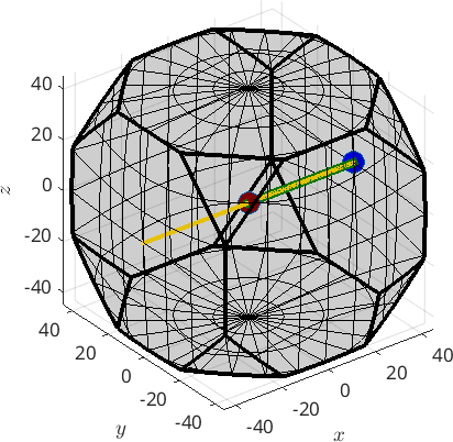
Fibres in pole figures and inverse pole figures
MTEX supports for fibers all the plotting options that are available for orientations. This included pole figures and inverse pole figures using the commands plotPDF and plotIPDF.
plotPDF(f,Miller({1,1,0},{1,1,1},cs),'linewidth',3,'lineColor','orange')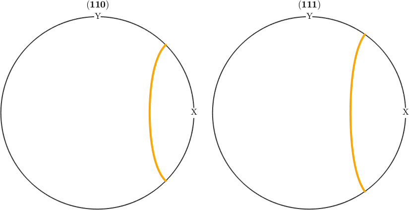
An important difference to orientation plots is that fibers are not automatically symmetrised when plotted. To achieve this use the command symmetrise.
plotPDF(f.symmetrise,Miller({1,1,0},{2,1,0},{1,1,1},cs),'linewidth',3,'lineColor','orange')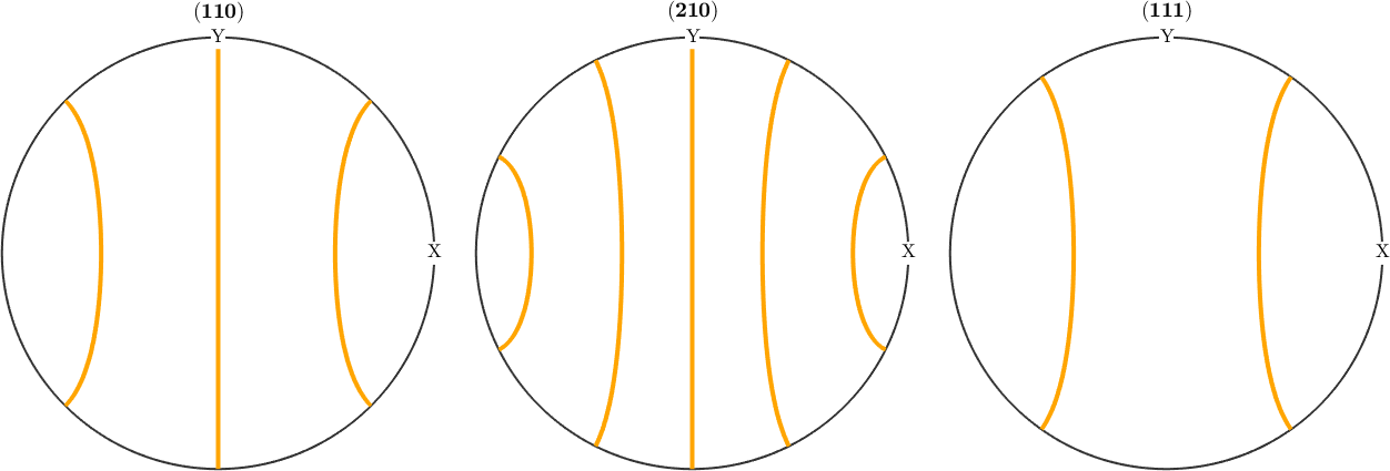
Inverse pole figures are by default restricted to the fundamental sector. You may use the option 'complete' to plot the entire sphere.
% an inverse pole figure plot
r = [vector3d(1,1,0),vector3d(2,1,0),vector3d(1,1,1)];
plotIPDF(f.symmetrise,r,'linewidth',3,'lineColor','orange')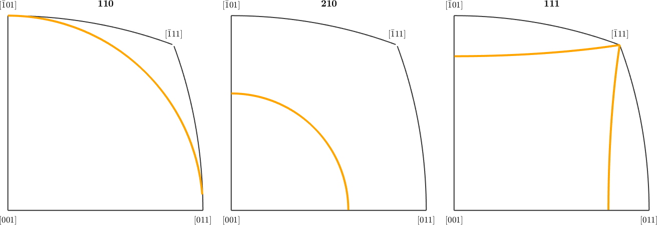
Defining a fibre by directions
Alternatively, a fibre can also be defined by a pair of a crystal and a specimen direction. In this case it consists of all orientations that aligns the crystal direction parallel to the specimen direction. As an example we define the fibre of all orientations such that the c-axis (001) is parallel to the z-axis by
f = fibre(Miller(0,0,1,cs),vector3d.Z)

plot(f,'linecolor','gold','linewidth',4,'project2FundamentalRegion','axisAngle')
f = fibre (432 → y↑→x)
h || r: (001) || (0,0,1)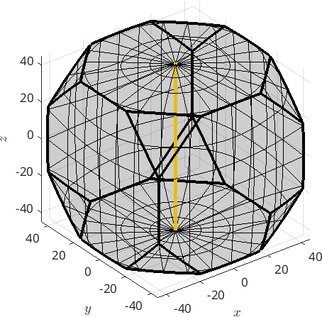
If both directions of type Miller the fibre corresponds to all misorientations which have these two direction parallel.
Finally, a fibre can be defined by an initial orientation ori1 and a direction h, i.e., all orientations ori of this fibre satisfy
ori * h = ori1 * hThe following code defines a fibre that passes through the cube orientation and rotates about the (111) axis.
f = fibre(ori1,Miller(1,1,1,cs))

plot(f,'linecolor','darkred','linewidth',4,'project2FundamentalRegion','axisAngle')
f = fibre (432 → y↑→x)
h || r: (111) || (1,1,1)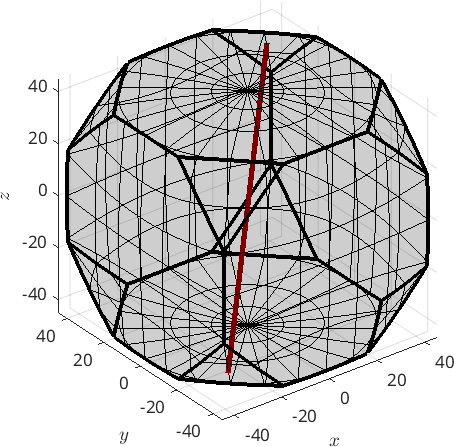
Predefined fibers
MTEX includes also a list of predefined fibers, e.g., alpha, beta, gamma, epsilon, eta, tau and theta fibers. Those can be defined by
ss = specimenSymmetry('orthorhombic');
beta = fibre.beta(cs,ss,'full')
beta = fibre (432 → y↑→x (mmm))
h || r: (12 6 11) || (1,1,4)
o1 → o2: (0°,35.3°,45°) → (0°,35.3°,45°)Lets plot an overview of all predefined fibers with respect to orthorhombic specimen symmetry
plot(fibre.alpha(cs,ss,'full'),'linewidth',3,'lineColor',ind2color(1),'DisplayName','alpha')
hold on
plot(fibre.beta(cs,ss,'full'),'linewidth',3,'lineColor',ind2color(2),'DisplayName','beta')
plot(fibre.gamma(cs,ss,'full'),'linewidth',3,'lineColor',ind2color(3),'DisplayName','gamma')
plot(fibre.epsilon(cs,ss,'full'),'linewidth',3,'lineColor',ind2color(4),'DisplayName','epsilon')
plot(fibre.eta(cs,ss,'full'),'linewidth',3,'lineColor',ind2color(5),'DisplayName','eta')
plot(fibre.tau(cs,ss,'full'),'linewidth',3,'lineColor',ind2color(6),'DisplayName','tau')
plot(fibre.theta(cs,ss,'full'),'linewidth',3,'lineColor',ind2color(7),'DisplayName','theta')
hold off
legend('Location','best')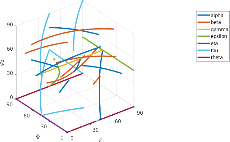
Fiber ODFs
Note, that it is straight forward to define a corresponding fibre ODF by the command fibreODF
odf = fibreODF(beta,'halfwidth',10*degree)

% and plot it in 3d
plot3d(odf)

% this adds the fibre to the plots
hold on
plot(beta.symmetrise,'lineColor','b','linewidth',4)
hold off
odf = SO3FunCBF (432 → y↑→x (mmm))
kernel: de la Vallee Poussin, halfwidth 10°
fibre : (12 6 11) || 1,1,4
weight: 1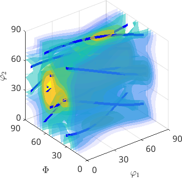
Visualize an ODF along a fibre
We may also visualize an ODF along a fibre
plot(odf,fibre.eta(cs,ss),'linewidth',2)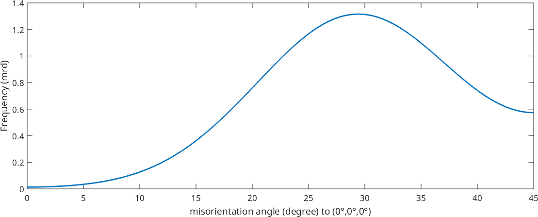
Compute volume of fibre portions
or compute the volume of an ODF in a tube around a fibre using the command volume
100 * volume(odf,beta,10*degree)ans =
100