
A grain combines several kinds of information: an identity, scalar properties, a mean orientation, an outline, and a place in the boundary network. No single exchange format on this page preserves all of them. Choose the representation that the receiving program needs, and record the information required to interpret it.
This page assumes that grains have already been reconstructed as in Grain Reconstruction. The examples use the Forsterite data set. Exporting a picture instead of the underlying data is covered in Exporting Plots.
plottingConvention.default('y↑→x');
mtexdata forsterite silent

grainsRaw = calcGrains(ebsd,'angle',10*degree);

% remove grains with ten or fewer measurements
grainsRaw = grainsRaw(grainsRaw.numPixel > 10)
grainsRaw = grain2d (y↑→x)
Phase Grains Pixels Mineral Symmetry Color
0 6 621 notIndexed none
1 443 151150 Forsterite mmm LightSkyBlue
2 184 25465 Enstatite mmm DarkSeaGreen
3 107 6962 Diopside 12/m1 Goldenrod
boundary segments: 43630 (2.1e+06 µm)
inner boundary segments: 173 (8052 µm)
triple points: 3403
Properties: meanRotation, GOSRecord how the grains were made
The displayed summary identifies the phases and the number of grains that will be exported. The cutoff above and the 10 degree reconstruction threshold are also part of the result. Record them with the source map, the MTEX version, and any other processing choices.
Smoothing changes polygon coordinates, areas, perimeters, and segment lengths. It does not change grain IDs, pixel counts, or mean orientations. We therefore keep grainsRaw for measurement-level boundary data and use a smoothed copy for shape data.
grains = smoothBoundary(grainsRaw,5);Export a grain table
A MATLAB table collects one row per grain. writetable can then write the rows to CSV for a spreadsheet or a statistics package.
A grain ID is a persistent label, not the row number in a subset. The distinction is demonstrated in Selecting Grains. The phase property is the numeric phase value imported with the map, so the readable mineral name is exported as a separate column. A grain with no data on one side of it has truncated geometry. The isBoundary column lets the receiver identify those grains instead of silently treating their visible area and perimeter as complete. Called with one argument, isBoundary flags every grain that owns a segment with no grain on the other side. That covers the grains at the map edge and the grains around an unindexed region inside the map. Passing the map as a second argument flags only the grains at its extent.
Lengths are in the map's measurement unit and areas in its square. This map uses micrometres, so the unit is included in each relevant column name. Shape Parameters defines these quantities. Any other scalar grain property can be appended in the same way.
mineralList = grains.mineralList;
mineral = reshape(string(mineralList(grains.phaseId)),[],1);

T = table(grains.id, grains.phase, mineral, grains.isBoundary, ...
  grains.numPixel, grains.area, grains.perimeter, ...
  grains.equivalentRadius, grains.GOS./degree, ...
  'VariableNames',{'id','phase','mineral','isBoundary','numPixel',...
  'area_um2','perimeter_um','equivalentRadius_um','GOS_degree'});

head(T)
id phase mineral isBoundary numPixel area_um2 perimeter_um equivalentRadius_um GOS_degree
__ _____ ____________ __________ ________ __________ ____________ ___________________ __________
19 1 "Forsterite" true 34 91250 1462.3 170.43 0.24256
21 2 "Enstatite" true 16 51473 1099.2 128 0.62956
22 1 "Forsterite" true 15 50640 996.04 126.96 0.42433
27 1 "Forsterite" true 19 55714 1056 133.17 0.17977
30 1 "Forsterite" true 26 72940 1156.8 152.37 0.28391
44 1 "Forsterite" true 51 2.0553e+05 2204.5 255.78 0.19108
53 1 "Forsterite" false 49 1.4646e+05 1600.2 215.92 0.48932
54 1 "Forsterite" false 23 65193 1081.5 144.05 0.4652Add mean orientations
An orientation row needs one crystal symmetry. We therefore restrict the table and both grain lists to Forsterite before adding Euler angles. Naming the Bunge convention and degree in the headings removes two common ambiguities.
grains = grains('Forsterite');
grainsRaw = grainsRaw('Forsterite');
T = T(T.mineral == "Forsterite",:);

[phi1,Phi,phi2] = grains.meanOrientation.Euler('Bunge');

T.phi1_Bunge_degree = phi1./degree;
T.Phi_Bunge_degree = Phi./degree;
T.phi2_Bunge_degree = phi2./degree;

csvFile = fullfile(tempdir,'grains.csv');
writetable(T,csvFile);

head(readtable(csvFile))
id phase mineral isBoundary numPixel area_um2 perimeter_um equivalentRadius_um GOS_degree phi1_Bunge_degree Phi_Bunge_degree phi2_Bunge_degree
__ _____ ______________ __________ ________ __________ ____________ ___________________ __________ _________________ ________________ _________________
19 1 {'Forsterite'} 1 34 91250 1462.3 170.43 0.24256 2.5813 161.36 269.26
22 1 {'Forsterite'} 1 15 50640 996.04 126.96 0.42433 133.37 168.62 247.12
27 1 {'Forsterite'} 1 19 55714 1056 133.17 0.17977 138.49 91.149 267.06
30 1 {'Forsterite'} 1 26 72940 1156.8 152.37 0.28391 33.863 82.646 349.95
44 1 {'Forsterite'} 1 51 2.0553e+05 2204.5 255.78 0.19108 123.16 80.504 260.91
53 1 {'Forsterite'} 0 49 1.4646e+05 1600.2 215.92 0.48932 165.83 107.25 260.95
54 1 {'Forsterite'} 0 23 65193 1081.5 144.05 0.4652 166.09 111.76 264.03
55 1 {'Forsterite'} 1 44 1.3889e+05 1615.5 210.26 0.62373 139.92 82.051 260.12The reloaded rows retain their values and descriptive headings. Adding the orientation columns makes the table self-contained only when the receiving program also knows the Forsterite crystal symmetry and the crystal and specimen reference frames. A reference frame is the frame in which the data are expressed.
A CSV file has no standard place for this context. Accompany it with a README or structured metadata that records the source, phase symmetries, spatial and angular units, Euler convention, reference frames, reconstruction threshold, size cutoff, and boundary smoothing.
Export mean orientations
When only the orientations are needed, export writes a compact ASCII table. Its conventions and limitations are described in Exporting Crystal Orientations.
orientationFile = fullfile(tempdir,'grainOrientations.txt');
export(grains.meanOrientation,orientationFile,'Bunge');

fid = fopen(orientationFile);
for k = 1:3, disp(fgetl(fid)); end
fclose(fid);
phi1 Phi phi2
2.58129 161.36 269.258
133.373 168.617 247.116The first line identifies the three Euler columns, and the following rows contain Bunge angles in degree. Crystal symmetry and reference frames are not stored in this file.
A struct appends one column per field. Every field must have one value per orientation, so grain properties remain aligned with their mean orientations.
S.area_um2 = grains.area;
S.GOS_degree = grains.GOS ./ degree;

export(grains.meanOrientation,orientationFile,S,'Bunge');

fid = fopen(orientationFile);
for k = 1:3, disp(fgetl(fid)); end
fclose(fid);
phi1 Phi phi2 area_um2 GOS_degree
2.58129 161.36 269.258 91250 0.242557
133.373 168.617 247.116 50640.4 0.424334Export a VPSC texture
export_VPSC writes the weighted texture format used by the VPSC crystal-plasticity code. It accepts Bunge, Kocks, or Roe Euler angles and normalises the supplied weights to sum to one.
Here the weights are observed areas on a two-dimensional section. Treating those area fractions as three-dimensional volume fractions is a modelling assumption, not a conversion performed by MTEX.
vpscFile = fullfile(tempdir,'grains.tex');
export_VPSC(grains.meanOrientation,vpscFile,'Bunge',...
  'weights',grains.area);

vpscData = readmatrix(vpscFile,'FileType','text','NumHeaderLines',4);
writtenWeightSum = sum(vpscData(:,4))
writtenWeightSum =
1.0000The printed sum is one to the precision stored in the text file. The VPSC header also records the Euler convention and number of orientations, but the phase symmetry and reference frames still need companion metadata.
Export polygon geometry
Each grain outline is stored as one or more closed loops. The property grains.poly contains vertex indices in walk order. These indices refer to grains.allV, the complete vertex list. They do not index grains.V, which is a shorter list containing only the vertices used by the current grain subset.
A grain that encloses another grain has an outer loop followed by one or more inner loops. This is the same enclosure described from the outside as a hole and from the inside as an inclusion. Each loop repeats its first vertex at the end.
V = grains.allV;
firstInterior = find(~grains.isBoundary,1);
poly = grains(firstInterior).poly{1};
polyVertexCount = numel(poly)

xy = [V(poly).x, V(poly).y];
xy(1:5,:)

newMtexFigure('figSize','small');
plot(grains(firstInterior),'FaceColor','LightSkyBlue','micronbar','off');
hold on
plot(xy(:,1),xy(:,2),'k.','MarkerSize',12);
hold off
polyVertexCount =
33
ans =
1.0e+03 *
0.3875 9.9000
0.3250 9.9000
0.2905 9.8809
0.2500 9.8500
0.2125 9.8125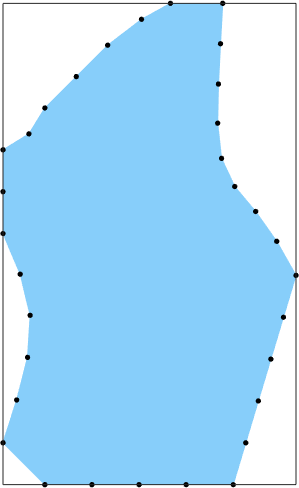
The blue area is the first grain that does not touch the map edge. The black markers trace the vertex walk that will be written, including the repeated endpoint that closes the loop. These are smoothed coordinates, not the original pixel staircase.
The following file contains every loop of every Forsterite grain. Both grainId and loopId are needed: a grain ID groups loops into grains, while a loop ID keeps an outer outline separate from enclosure outlines.
polygonFile = fullfile(tempdir,'grainPolygons.txt');
fid = fopen(polygonFile,'w');
fprintf(fid,'%% grainId loopId x_um y_um\n');
for k = 1:length(grains)
  p = grains(k).poly{1};
  loopStart = 1;
  loopId = 1;
  while loopStart < numel(p)
    loopEnd = loopStart + find(p(loopStart+1:end) == p(loopStart),1);
    q = p(loopStart:loopEnd);
    fprintf(fid,'%d %d %.17g %.17g\n',...
      [repmat(double(grains.id(k)),1,numel(q)); ...
      repmat(loopId,1,numel(q)); V(q).x.'; V(q).y.']);
    loopStart = loopEnd + 1;
    loopId = loopId + 1;
  end
end
fclose(fid);

fid = fopen(polygonFile);
for k = 1:4, disp(fgetl(fid)); end
fclose(fid);
% grainId loopId x_um y_um
19 1 100 11799.999999999998
19 1 58.333333333401242 11808.333333333336
19 1 16.666666666813388 11816.666666666672Export the boundary network
A grain boundary is a segment between two neighbouring EBSD measurements that belong to different grains. The boundary table below uses the unsmoothed network so each row retains that measurement-level meaning. It excludes segments next to grains removed by the size cutoff.
gB = grainsRaw.boundary('Forsterite','Forsterite');
gB = gB(all(ismember(gB.grainId,grainsRaw.id),2));

TB = table(gB.grainId(:,1),gB.grainId(:,2),gB.segLength,...
  gB.misorientation.angle./degree,...
  'VariableNames',{'grainA','grainB','segLength_um',...
  'segmentDisorientation_degree'});

head(TB)
grainA grainB segLength_um segmentDisorientation_degree
______ ______ ____________ ____________________________
937 972 35.355 26.131
937 972 50 26.086
2645 2696 46.585 24.156
2645 2696 27.951 23.605
2645 2696 25 23.571
2645 2696 35.355 23.823
2645 2696 50 23.646
2645 2696 35.355 23.976 gB stores one row per boundary segment. The two IDs identify its neighbouring grains. The angle is the disorientation between the adjacent measurements across that segment, not the disorientation between the two grain mean orientations. Continue with Grain Boundary Properties before exporting further segment quantities.
Save MTEX objects
If the data will be read by the same MTEX installation, MATLAB save preserves the complete objects more conveniently than separate text tables. Saving the source map with both grain lists keeps the measurements available for later checks; the processing history still belongs in the companion metadata.
matFile = fullfile(tempdir,'grains.mat');
save(matFile,'grains','grainsRaw','ebsd');
The MTEX objects inside a .mat file are not readable by general non-MATLAB software, and they are not guaranteed to load in a future MTEX version. For long-term archiving, prefer documented ASCII tables such as those above together with the source data and companion metadata. No one of these tables replaces the complete MTEX objects.
Remove the temporary files created by this page.
delete(csvFile);
delete(orientationFile);
delete(vpscFile);
delete(polygonFile);
delete(matFile);
Further reading
- ISO 13067:2020, Microbeam analysis - Electron backscatter diffraction - Measurement of average grain size, distinguishes measurements on a two-dimensional section from inferences about three-dimensional grain size.
- H.-J. Bunge, Texture Analysis in Materials Science: Mathematical Methods, Butterworths, English ed., 1982, establishes the Euler-angle convention used in texture analysis.
- R. A. Lebensohn and C. N. Tomé, A self-consistent anisotropic approach for the simulation of plastic deformation and texture development of polycrystals, Acta Metallurgica et Materialia 41 (1993), 2611-2624, introduces the VPSC formulation.
- M. D. Wilkinson et al., The FAIR Guiding Principles for scientific data management and stewardship, Scientific Data 3 (2016), 160018, explains why reusable data need rich metadata and provenance.
Next
Neper Interface follows this page in the chapter and constructs synthetic polycrystals for simulation. For measured grain boundaries, continue with Grain Boundaries.
Citing this page.
This page is part of the documentation of
MTEX, a free and open
source MATLAB toolbox for analyzing and modeling crystallographic textures.
It was written by The MTEX Developers and is published at
https://mtex-toolbox.github.io/GrainExport.html.
If you use MTEX, or reuse text or figures from this page, in your research,
please cite
F. Bachmann, R. Hielscher, H. Schaeben: Texture Analysis with MTEX - Free and Open Source Software Toolbox, Solid State Phenomena 160 (2010), 63-68. 10.4028/www.scientific.net/SSP.160.63
BibTeX
@article{bachmann2010mtex,
  author  = {F. Bachmann and R. Hielscher and H. Schaeben},
  title   = {Texture Analysis with MTEX - Free and Open Source Software Toolbox},
  journal = {Solid State Phenomena},
  volume  = {160},
  pages   = {63-68},
  year    = {2010},
  doi     = {10.4028/www.scientific.net/SSP.160.63},
  url     = {https://doi.org/10.4028/www.scientific.net/SSP.160.63}
}
Other papers describing specific MTEX methods are listed under Publications — please cite the one that best fits your application. The MTEX source code is licensed under the GNU General Public License v2.0; the text and figures of this documentation are licensed under CC BY 4.0, which permits reuse — including by automated systems — provided The MTEX Developers and this page are credited.