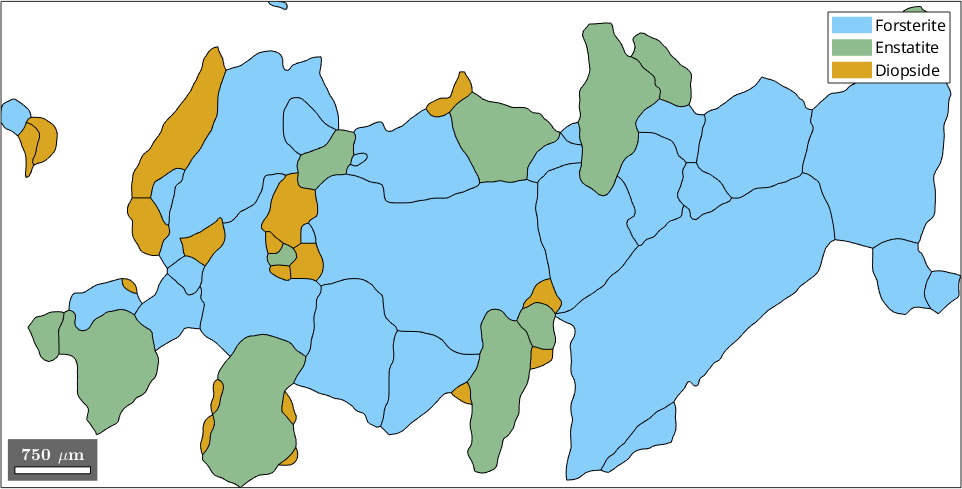
In this section we discuss how to select grains by properties. We start our discussion by reconstructing the grain structure from a sample EBSD data set.
% load sample EBSD data set
mtexdata forsterite silent

% restrict it to a subregion of interest.
ebsd = ebsd(inpolygon(ebsd,[5 2 10 5]*10^3));

% remove all not indexed pixels
ebsd = ebsd('indexed');

% reconstruct grains
[grains, ebsd.grainId] = calcGrains(ebsd,'angle',5*degree,'minPixel',5);

% smooth them
grains = smooth(grains,5);

% plot the orientation data of the Forsterite phase
plot(ebsd('fo'),ebsd('fo').orientations)

% plot the grain boundary on top of it
hold on
plot(grains.boundary,'lineWidth',2)
hold off
Selecting grains by mouse
The most easiest way to select a grain is by using the mouse and the command selectInteractive which allows you to select an arbitrary amount of grains. The index of the selected grains appear as the global variable indSelected in your workspace
selectInteractive(grains,'lineColor','gold')

% this simulates a mouse click
pause(1)
simulateClick(9000,3500)
pause(1)

global indSelected;
grains(indSelected)

hold on
plot(grains(indSelected).boundary,'lineWidth',4,'lineColor','gold')
hold off
Grain selected: 92
ans = grain2d (y↑→x)
Phase Grains Pixels Mineral Symmetry Color
1 1 235 Forsterite mmm LightSkyBlue
boundary segments: 135 (5521 µm)
inner boundary segments: 1 (12 µm)
triple points: 5
Id Phase Pixels meanRotation GOS
92 1 235 (181°,152°,258°) 0.0137728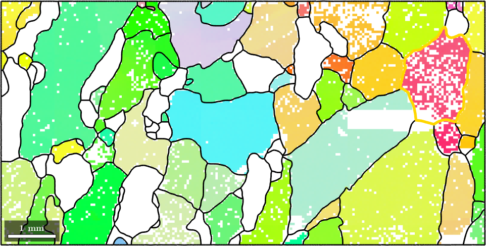
Indexing by orientation or position
One can also to select a grain by spatial coordinates without user interaction. This is done using the syntax grains(x,y), i.e.,
x = 12000; y = 4000;

hold on
plot(grains(x,y).boundary,'linewidth',4,'linecolor','blue')

plot(x,y,'marker','s','markerfacecolor','k',...
  'markersize',10,'markeredgecolor','w')
hold off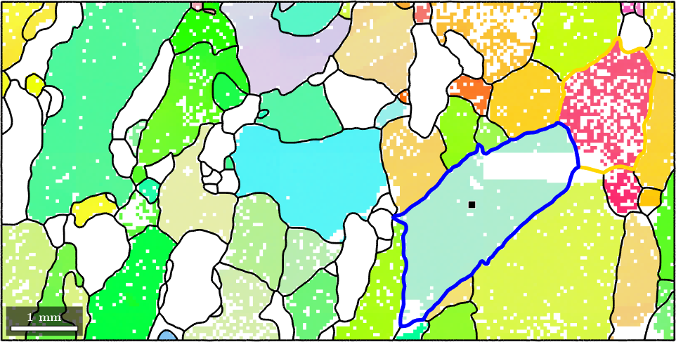
Alternatively one can also select all grains with a certain orientation. Lets find all grains with a similar orientation as the one marked in gold. As threshold we shall use 20 degree
% select grains by orientation
grains_selected = grains.findByOrientation(grains(indSelected).meanOrientation,20*degree)

hold on
plot(grains_selected.boundary,'linewidth',4,'linecolor','gold')
hold off
grains_selected = grain2d (y↑→x)
Phase Grains Pixels Mineral Symmetry Color
1 7 1140 Forsterite mmm LightSkyBlue
boundary segments: 599 (23014 µm)
inner boundary segments: 1 (12 µm)
triple points: 24
Id Phase Pixels meanRotation GOS
11 1 63 (177°,140°,249°) 0.013
52 1 321 (177°,146°,251°) 0.014
60 1 7 (13°,13°,266°) 0.0084
68 1 258 (166°,147°,259°) 0.018
79 1 123 (14°,42°,279°) 0.041
92 1 235 (181°,152°,258°) 0.014
96 1 133 (1°,47°,279°) 0.0083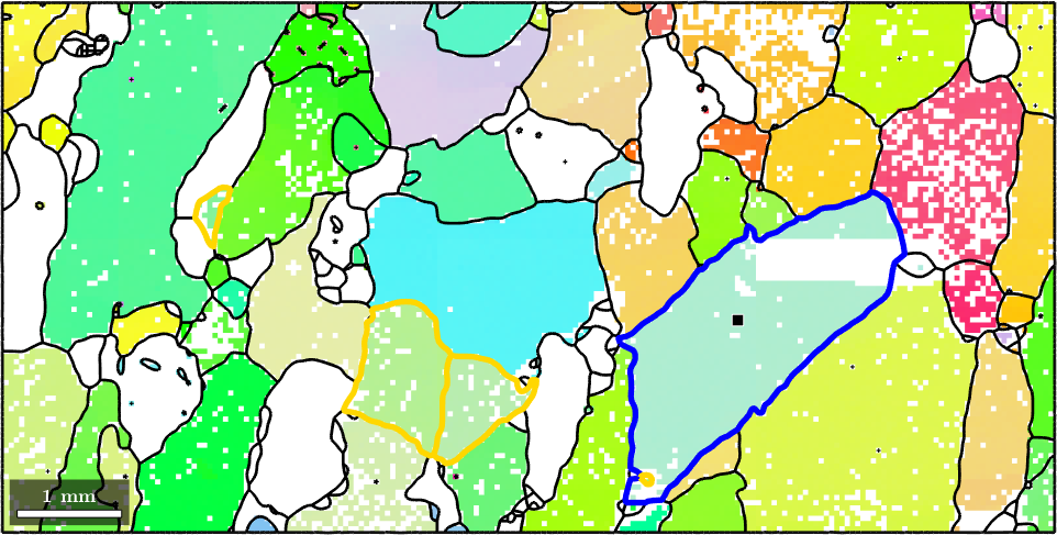
Indexing by a Property
In order the generalize the above concept lets remember that the variable grains is essentially a large vector of grains. Thus when applying a function like area to this variable we obtain a vector of the same length with numbers representing the area of each grain
grain_area = grains.area;As a first rather simple application we could colorize the grains according to their area, i.e., according to the numbers stored in grain_area
plot(grains,grain_area)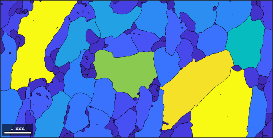
As a second application, we can ask for the largest grain within our data set. The maximum value and its position within a vector are found by the MATLAB command max.
[max_area,max_id] = max(grain_area)max_area =
4.1272e+06
max_id =
38The number max_id is the position of the grain with a maximum area within the variable grains. We can access this specific grain by direct indexing
grains(max_id)ans = grain2d (y↑→x)
Phase Grains Pixels Mineral Symmetry Color
1 1 1448 Forsterite mmm LightSkyBlue
boundary segments: 222 (8622 µm)
inner boundary segments: 0 (0 µm)
triple points: 5
Id Phase Pixels meanRotation GOS
38 1 1448 (166°,127°,259°) 0.0135419and so we can plot it
hold on
plot(grains(max_id).boundary,'linecolor','red','linewidth',4)
hold off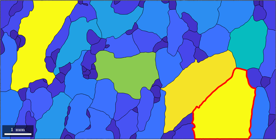
Note that this way of addressing individual grains can be generalized to many grains. E.g. assume we are interested in the largest 5 grains. Then we can sort the vector grain_area and take the indices of the 5 largest grains.
[sorted_area,sorted_id] = sort(grain_area,'descend');

large_grain_id = sorted_id(2:5);

hold on
plot(grains(large_grain_id).boundary,'linecolor','Orange','linewidth',4)
hold off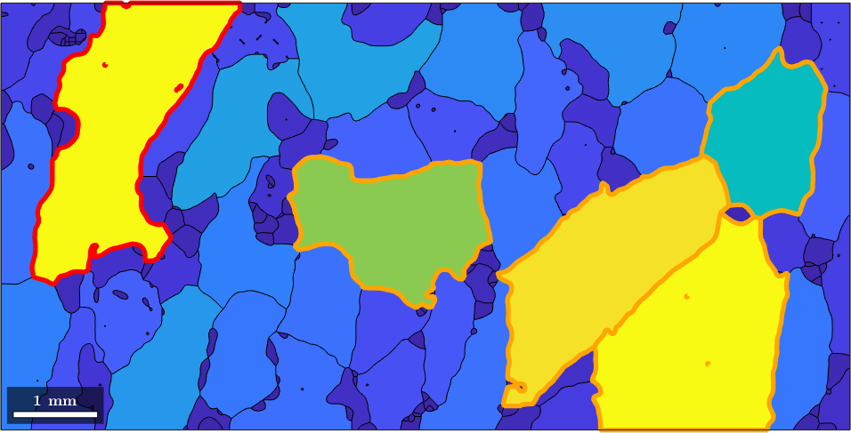
Indexing by a Condition
By the same syntax as above we can also single out grains that satisfy a certain condition. I.e., to access are grains that are at least one quarter as large as the largest grain we can do
condition = grain_area > max_area/4;

hold on
plot(grains(condition).boundary,'linecolor','Yellow','linewidth',4)
hold off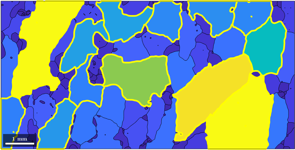
This is a very powerful way of accessing grains as the condition can be build up using any grain property. As an example let us consider the phase. The phase of the first five grains we get by
grains(1:5).phaseans =
1
3
1
3
3Now we can access or grains of the first phase Forsterite by the condition
condition = grains.phase == 1;
plot(grains(condition))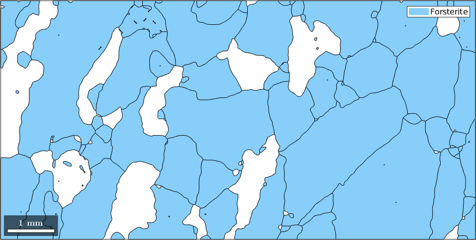
To make the above more directly you can use the mineral name for indexing
grains('forsterite')ans = grain2d (y↑→x)
Phase Grains Pixels Mineral Symmetry Color
1 61 14010 Forsterite mmm LightSkyBlue
boundary segments: 3543 (134904 µm)
inner boundary segments: 15 (317 µm)
triple points: 136
Properties: meanRotation, GOSLogical indexing allows also for more complex queries, e.g. selecting all grains perimeter larger than 6000 and at least 600 measurements within
condition = grains.perimeter>6000 & grains.numPixel >= 600;

selected_grains = grains(condition)

plot(selected_grains)
selected_grains = grain2d (y↑→x)
Phase Grains Pixels Mineral Symmetry Color
1 4 5248 Forsterite mmm LightSkyBlue
boundary segments: 886 (34740 µm)
inner boundary segments: 0 (0 µm)
triple points: 43
Id Phase Pixels meanRotation GOS
38 1 1448 (166°,127°,259°) 0.014
47 1 1047 (89°,99°,224°) 0.0077
50 1 1208 (153°,68°,237°) 0.0081
82 1 1545 (167°,81°,251°) 0.013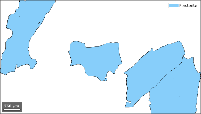
The grainId and how to select EBSD inside specific grains
Besides, the list of grains the command calcGrains returns also two other output arguments.
plot(grains)
largeGrains = grains(grains.numPixel > 50);

text(largeGrains,largeGrains.id)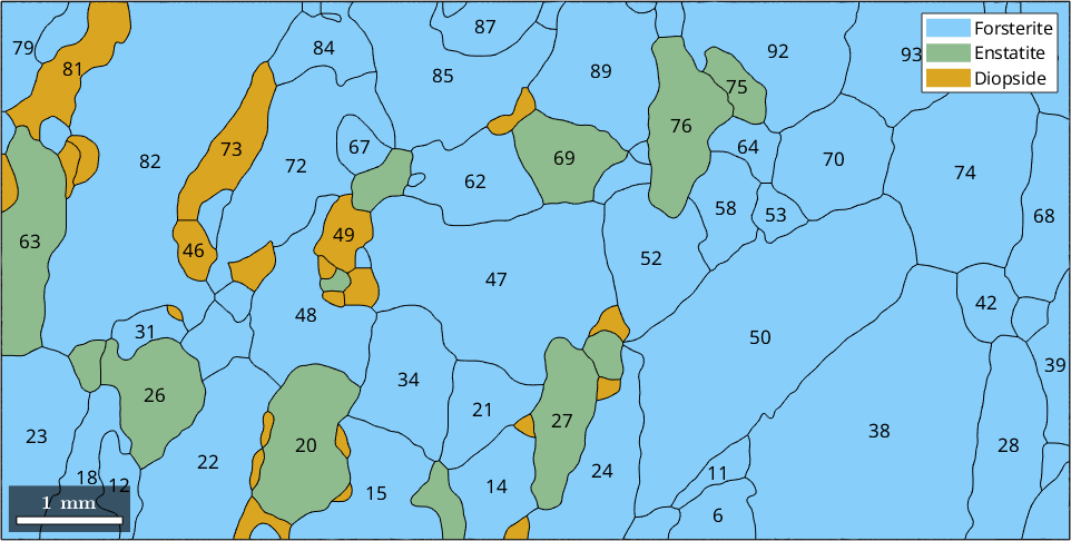
The second output argument grainId is a list with the same size as the EBSD measurements that stores for each measurement the corresponding grainId. The above syntax stores this list directly inside the ebsd variable. This enables MTEX to select EBSD data by grains. The following command returns all the EBSD data that belong to grain number 33.
ebsd(grains(33))ans = EBSD (y↑→x)
Phase Orientations Mineral Color Symmetry Crystal reference frame
1 42 (100%) Forsterite LightSkyBlue mmm
Properties: bands, bc, bs, error, mad, grainId
Scan unit : um
X x Y x Z : [6750, 7300] x [3550, 4150] x [0, 0]
Normal vector: (0,0,1)and is equivalent to the command
ebsd(ebsd.grainId == 33)ans = EBSD (y↑→x)
Phase Orientations Mineral Color Symmetry Crystal reference frame
1 42 (100%) Forsterite LightSkyBlue mmm
Properties: bands, bc, bs, error, mad, grainId
Scan unit : um
X x Y x Z : [6750, 7300] x [3550, 4150] x [0, 0]
Normal vector: (0,0,1)The following picture plots the largest grains together with its individual orientation measurements.
plot(ebsd(grains(max_id)),ebsd(grains(max_id)).orientations)
hold on
plot(grains(max_id).boundary,'lineWidth',2)
hold off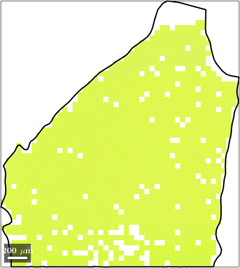
Boundary grains
Sometimes it is desirable to remove all boundary grains as they might distort grain statistics. To do so one should remember that each grain boundary has a property grainId which stores the ids of the neighboring grains. In the case of an outer grain boundary, one of the neighboring grains has the id zero. We can filter out all these boundary segments by
% ids of the outer boundary segment
outerBoundary_id = any(grains.boundary.grainId==0,2);

% plot the outer boundary segments
plot(grains)
hold on
plot(grains.boundary(outerBoundary_id),'linecolor','red','linewidth',2)
hold off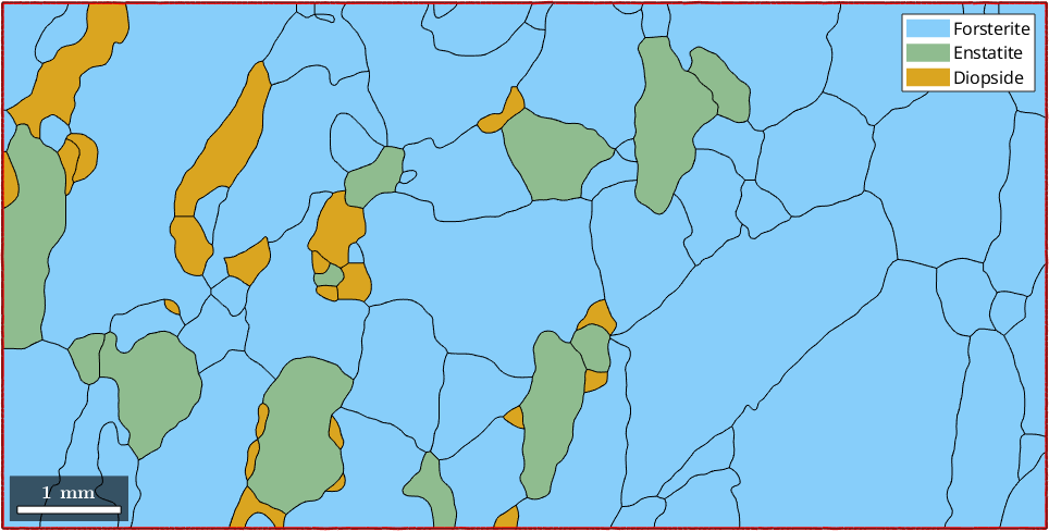
Now grains.boundary(outerBoundary_id).grainId is a list of grain ids where the first column is zero, indicating the outer boundary, and the second column contains the id of the boundary grain. Hence, it remains to remove all grains with these ids.
% next we compute the corresponding grain_id
grain_id = grains.boundary(outerBoundary_id).grainId;

% remove all zeros
grain_id(grain_id==0) = [];

% and plot the boundary grains
plot(grains(grain_id))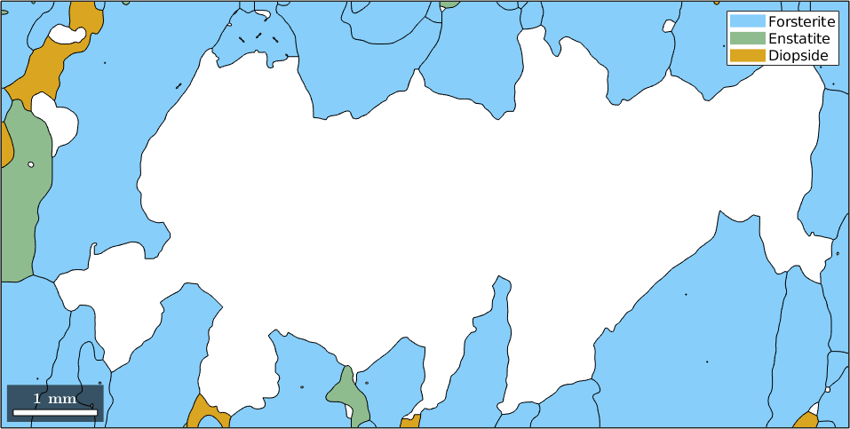
finally, we could remove the boundary grains by
grains(grain_id) = []However, boundary grains can be selected more easily be the command isBoundary.
plot(grains(~grains.isBoundary))