This script demonstrates the tools MTEX offers to reconstruct a parent austenite phase from a measured martensite phase. Most of the ideas are from Crystallography, Morphology, and Martensite Transformation of Prior Austenite in Intercritically Annealed High-Aluminum Steel by Tuomo Nyyssönen. We shall use the following sample data set.
% load the data
mtexdata martensite
% extract fcc and bcc symmetries
csBCC = ebsd.CSList{2}; % austenite bcc:
csFCC = ebsd.CSList{3}; % martensite fcc:
% grain reconstruction
[grains,ebsd.grainId] = calcGrains(ebsd('indexed'),'angle',3*degree,'minPixel',5);
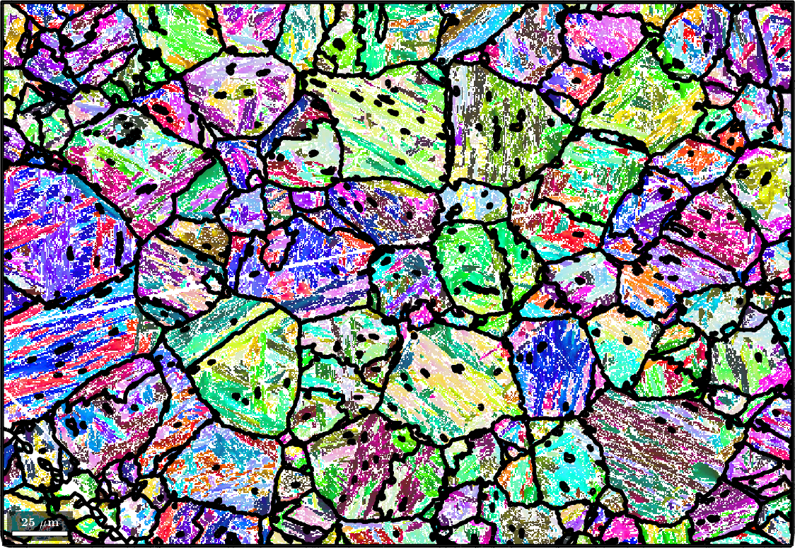
% plot the data and the grain boundaries
plot(ebsd('Iron bcc'),ebsd('Iron bcc').orientations,'figSize','large')
hold on
plot(grains.boundary,'linewidth',2)
hold offebsd = EBSD (y↑→x)
Phase Orientations Mineral Color Symmetry Crystal reference frame
0 92415 (27%) notIndexed
1 251187 (73%) Iron bcc (old) LightSkyBlue 432
Properties: bands, bc, bs, error, mad, reliabilityindex
Scan unit : um
X x Y x Z : [0, 353] x [0, 242] x [0, 0]
Normal vector: (0,0,1)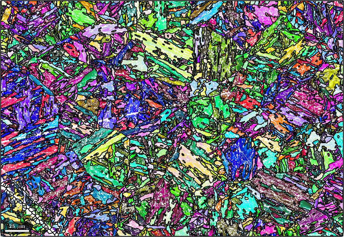
Determine the parent child orientation relationship
It is well known that the phase transformation from austenite to martensite is not described by a fixed orientation relationship. In fact, the actual orientation relationship needs to be determined for each sample individually. Here, we used the iterative method proposed by Tuomo Nyyssönen and implemented in the function calcParent2Child that starts at an initial guess of the orientation relation ship and iterates towards the true orientation relationship.
Here we use as the initial guess the Kurdjumov Sachs orientation relationship
% initial gues is Kurdjumov Sachs
KS = orientation.KurdjumovSachs(csFCC,csBCC);
The function calcParent2Child requires as input a list of child to child misorientations or, equivalently, a two column matrix of child orientations. Here we go with the second option and setup this two column orientation matrix from the mean orientations of neighboring grains which can be found using the command neighbours
% get neighboring grain pairs
grainPairs = grains.neighbors;

% ignore pairs with misorientation angle smaller then 5 degree
mori = grains(grainPairs).meanOrientation;
grainPairs(angle(mori(:,1),mori(:,2)) < 5*degree,:) = [];

% compute an optimal parent to child orientation relationship
[fcc2bcc, fit] = calcParent2Child(grains(grainPairs).meanOrientation,KS);
Beside the optimized parent to child orientation relationship the command calcParent2Child returns as a second output argument the misfit between all grain to grain misorientations and the theoretical child to child misorientations. In fact, the algorithm assumes that the majority of all boundary misorientations are child to child misorientations and finds the parent to child orientations relationship by minimizing this misfit. The following histogram displays the distribution of the misfit over all grain to grain misorientations.
close all
histogram(fit./degree)
xlabel('disorientation angle')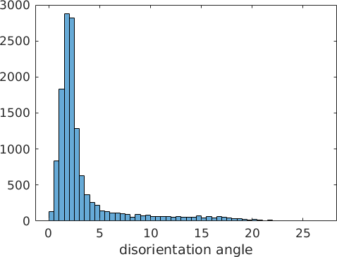
We may also colorize the grain boundaries according to this misfit. To this end we first compute the relationship between pairs of grains grainPairs and the boundary segments stored in grains.boundary using the command selectByGrainId
[gB,pairId] = grains.boundary.selectByGrainId(grainPairs);and then pass the variable fit as second input argument to the plot command
plot(ebsd('Iron bcc'),ebsd('Iron bcc').orientations,'figSize','large')
hold on;
plot(gB,fit(pairId) ./ degree,'linewidth',3,'smooth')
hold off

mtexColorMap LaboTeX
mtexColorbar

setColorRange([0,5])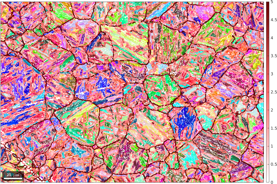
We observe that the boundary segments with a large misfit form large grain shapes which we want to identify in the next steps as the parent grains.
Create a similarity matrix
Next we set up a adjacency matrix A that describes the probability that two neighboring grains belong to the same parent grains. This probability is computed from the misfit of the misorientation between two child grains to the theoretical child to child misorientation. More precisely, we model the probability by a cumulative Gaussian distribution with the mean value threshold which describes the misfit at which the probability is exactly 50 percent and the standard deviation tol
omega = linspace(0,5)*degree;
threshold = 2*degree;
tol = 1.5*degree;

close all
plot(omega./degree,1 - 0.5 * (1 + erf(2*(omega - threshold)./tol)),'linewidth',2)
xlabel('misfit in degree')
ylabel('probability')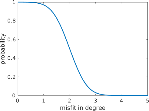
The above diagram describes the probability distribution as a function of the misfit. After filling the matrix A with these probabilities
% compute the probabilities
prob = 1 - 0.5 * (1 + erf(2*(fit - threshold)./tol));

% the corresponding similarity matrix
A = sparse(grainPairs(:,1),grainPairs(:,2),prob,length(grains),length(grains));
we can split it into clusters using the command calcCluster which implements the Markovian clustering algorithm. Here an important parameter is the so called inflation power, which controls the size of the clusters.
p = 1.6; % inflation power:
A = mclComponents(A,p);
Each connected component of the resulting adjacency matrix describes one parent grain. Hence, we can use this adjacency matrix to merge child grains into parent grains by the command merge.
% merge grains according to the adjacency matrix A
[parentGrains, parentId] = merge(grains,A);

% ensure grainId in parentEBSD is set up correctly with parentGrains
parentEBSD = ebsd;
parentEBSD('indexed').grainId = parentId(ebsd('indexed').grainId);
Let's visualize the first result. Note, that at this stage it is not important to have the parent grains already at their optimal size. Similarly orientated grains can be merged later on.
plot(ebsd('Iron bcc'),ebsd('Iron bcc').orientations,'figSize','large')
hold on;
plot(parentGrains.boundary,'linewidth',4,'lineColor','w')
plot(parentGrains.boundary,'linewidth',2,'lineColor','k')
hold off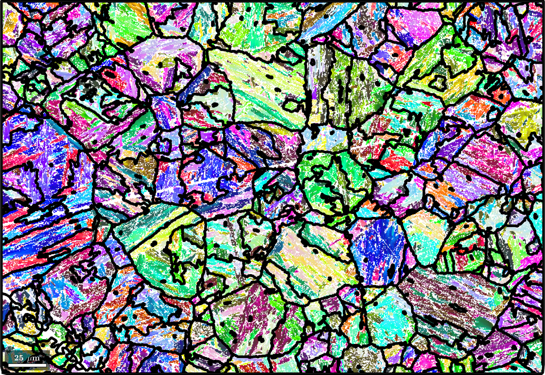
Compute parent grain orientations
In the next step we compute for each parent grain its parent austenite orientation. This can be done usig the command calcParent. Note, that we ensure that at least two child grains have been merged and that the misfit is smaller than 5 degree.
% the measured child orientations
childOri = grains('Iron bcc').meanOrientation;

% the parent orientation we are going to compute
parentOri = orientation.nan(max(parentId),1,fcc2bcc.CS);
fit = inf(size(parentOri));
weights = grains('Iron bcc').numPixel;

% loop through all parent grains
pC = progressCounter(max(parentId));
for k = 1:max(parentId)
  if nnz(parentId==k) > 1
    % compute the parent orientation from the child orientations
    [parentOri(k),fit(k)] = calcParent(childOri(parentId==k), fcc2bcc,'weights',weights((parentId==k)));
  end
  pC.show(k);
end

% update mean orientation of the parent grains
parentGrains(fit<5*degree).meanOrientation = parentOri(fit<5*degree);
parentGrains = parentGrains.update;

% merge grains with similar orientation
[parentGrains, mergeId] = merge(parentGrains,'threshold',4*degree);
parentEBSD('indexed').grainId = mergeId(parentEBSD('indexed').grainId);
Let's plot the resulting parent orientations
plot(parentGrains('Iron fcc'),parentGrains('Iron fcc').meanOrientation)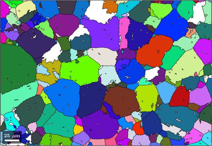
Compute Child Variants
Knowing the parent grain orientations we may compute the |variantId| of each child grain using the command calcVariantId. As a bonus this command returns also the packetId, here defined as the closest {111} plane in austenite to the (011) plane in martensite.
% compute variantId and packetId
[variantId,packetId] = calcVariantId(parentOri(parentId),childOri,fcc2bcc);

% associate to each packet id a color and plot
color = ind2color(packetId);
plot(grains,color)

hold on
plot(parentGrains.boundary,'linewidth',3)

% outline a specific parent grain
hold on
id = parentGrains.findByLocation([100,80]);
plot(parentGrains(id).boundary,'linewidth',3,'lineColor','w')
hold off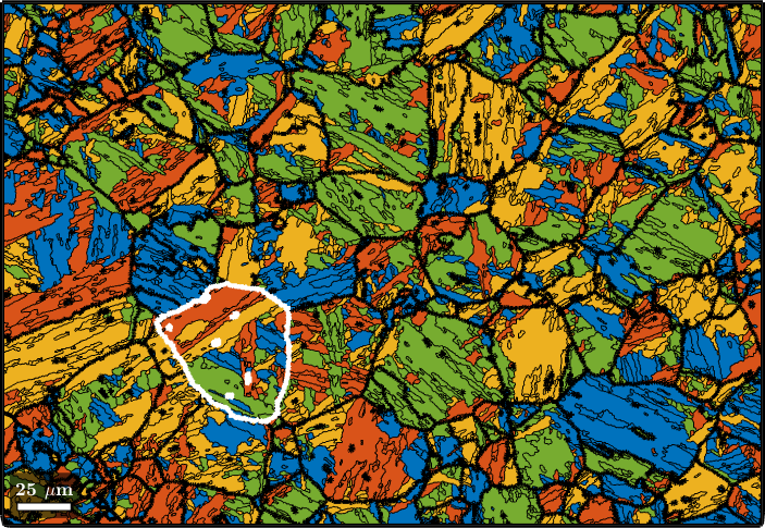
In order to check our parent grain reconstruction we chose the single parent grain outlines in the above map and plot all child variants of its reconstructed parent orientation together with the actually measured child orientations inside the parent grain.
% the measured child orientations that belong to parent grain 279
childOri = ebsd(parentEBSD.grainId==id).orientations;
plotPDF(childOri,Miller(0,0,1,csBCC),'MarkerSize',3)

% the orientation of parent grain 279
hold on
parentOri = parentGrains(id).meanOrientation;
plot(parentOri.symmetrise * Miller(0,0,1,csFCC))

% the theoretical child variants
childVariants = variants(fcc2bcc, parentOri);
plotPDF(childVariants, 'markerFaceColor','none','linewidth',2,'markerEdgeColor','orange')
hold off
I'm plotting 416 random orientations out of 6841 given orientations
You can specify the the number points by the option "points".
The option "all" ensures that all data are plotted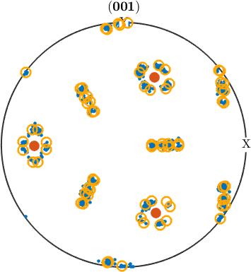
So far our analysis was at the grain level. However, once parent grain orientations have been computed we may also use them to compute parent orientations of each pixel in our original EBSD map. To this end we first find pixels that now belong to an austenite grain.
% consider only martensite pixels that now belong to austenite grains
isNowFCC = parentGrains.phaseId(max(1,parentEBSD.grainId)) == 3 & parentEBSD.phaseId == 2;

% compute parent orientation
[parentEBSD(isNowFCC).orientations, fit] = calcParent(ebsd(isNowFCC).orientations,...
  parentGrains(parentEBSD(isNowFCC).grainId).meanOrientation,fcc2bcc);

% plot the result
plot(parentEBSD('Iron fcc'),parentEBSD('Iron fcc').orientations,'figSize','large')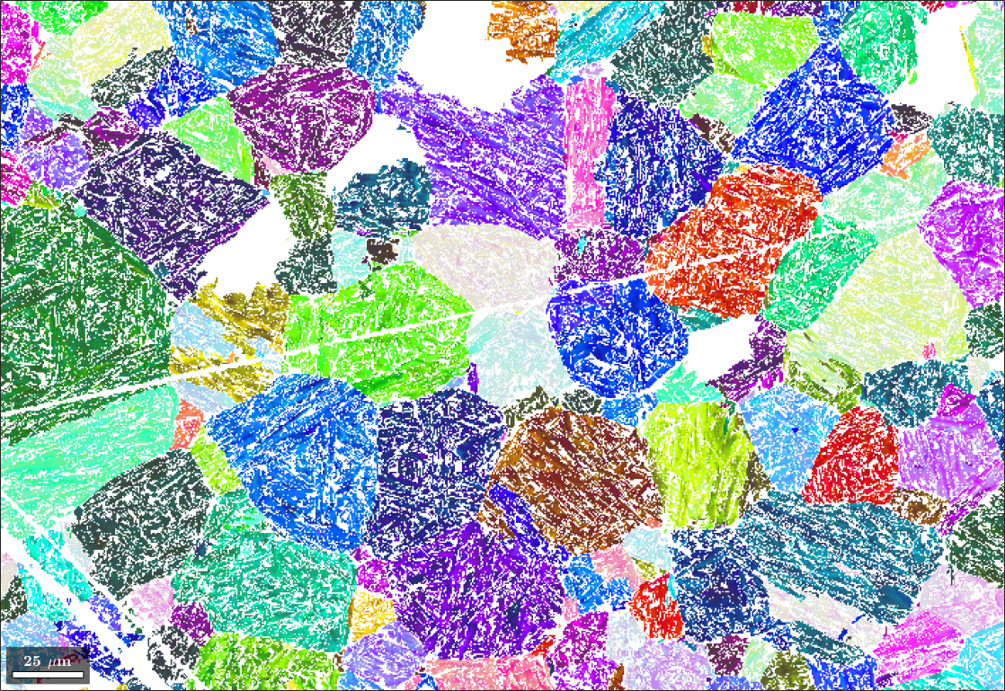
As a second output argument we obtain the misfit between the parent orientation computed for the pixel and the mean orientation of the corresponding parent grain. Let's plot this misfit as a map.
plot(parentEBSD(isNowFCC),fit ./ degree,'figSize','large')
mtexColorMap LaboTeX
mtexColorbar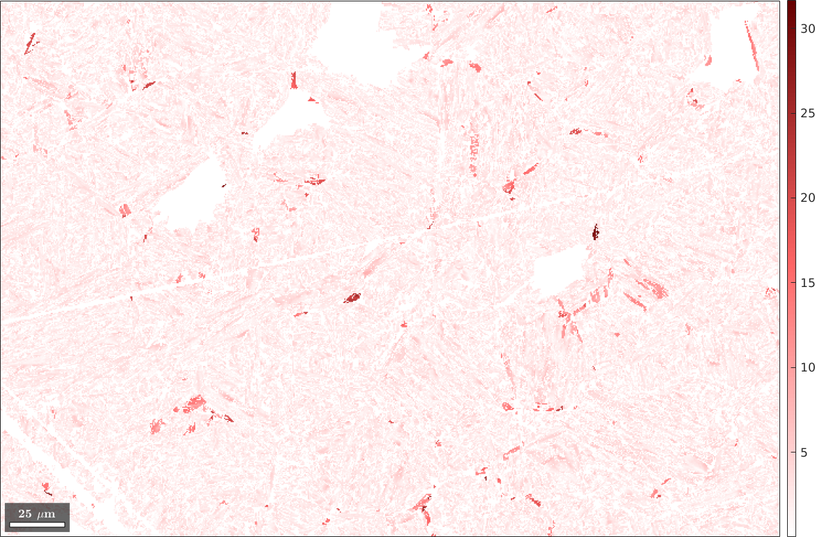
Denoise the parent map
Finaly we may apply filtering to the parent map to fill non indexed or not reconstructed pixels. To this end we first run grain reconstruction on the parent map
[parentGrains, parentEBSD.grainId] = ...
  calcGrains(parentEBSD('indexed'),'angle',3*degree,'minPixel',10);

parentGrains = smooth(parentGrains,5);

plot(ebsd('indexed'),ebsd('indexed').orientations,'figSize','large')

hold on
plot(parentGrains.boundary,'lineWidth',4)
hold off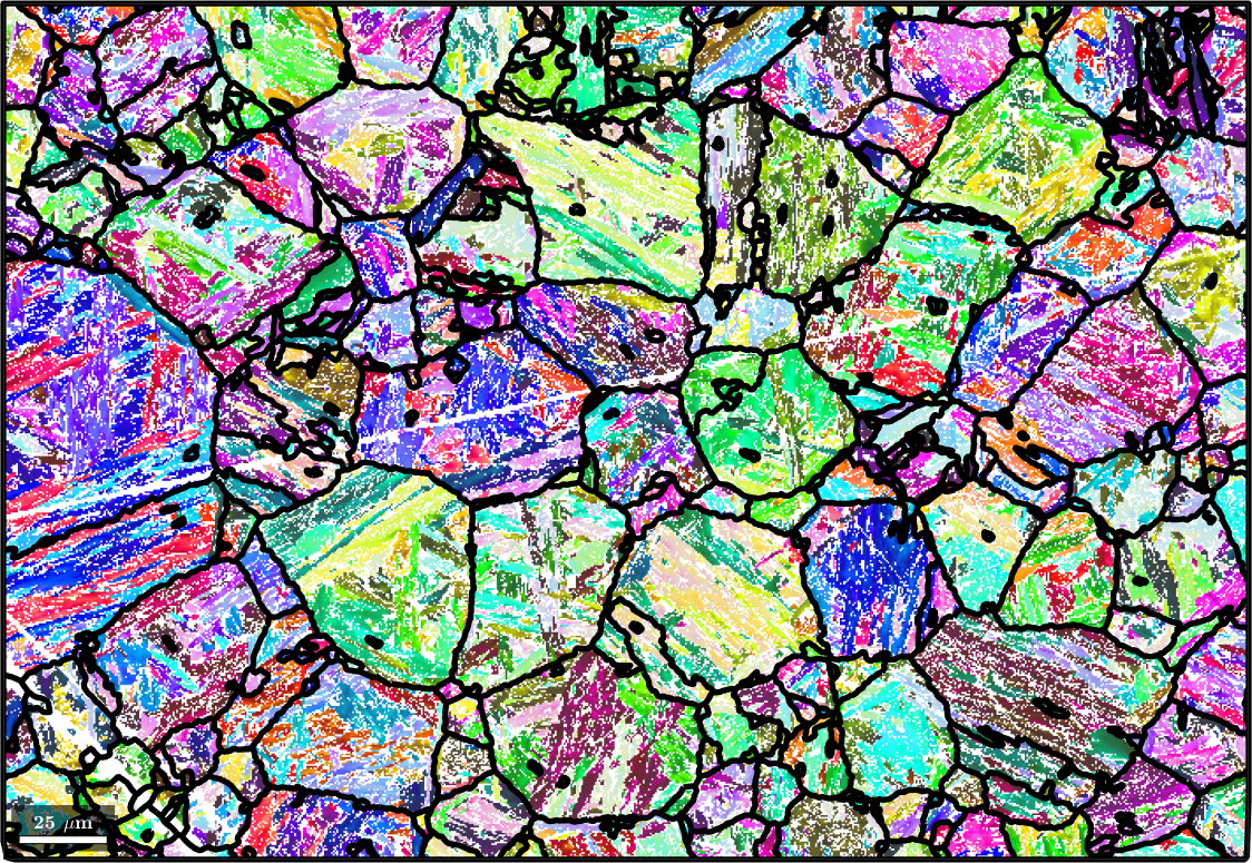
and then use the command smooth to fill the holes in the reconstructed parent map
% fill the holes
F = halfQuadraticFilter;
parentEBSD = smooth(parentEBSD('indexed'),F,'fill',parentGrains);

% plot the parent map
plot(parentEBSD('Iron fcc'),parentEBSD('Iron fcc').orientations,'figSize','large')

% with grain boundaries
hold on
plot(parentGrains.boundary,'lineWidth',4)
hold off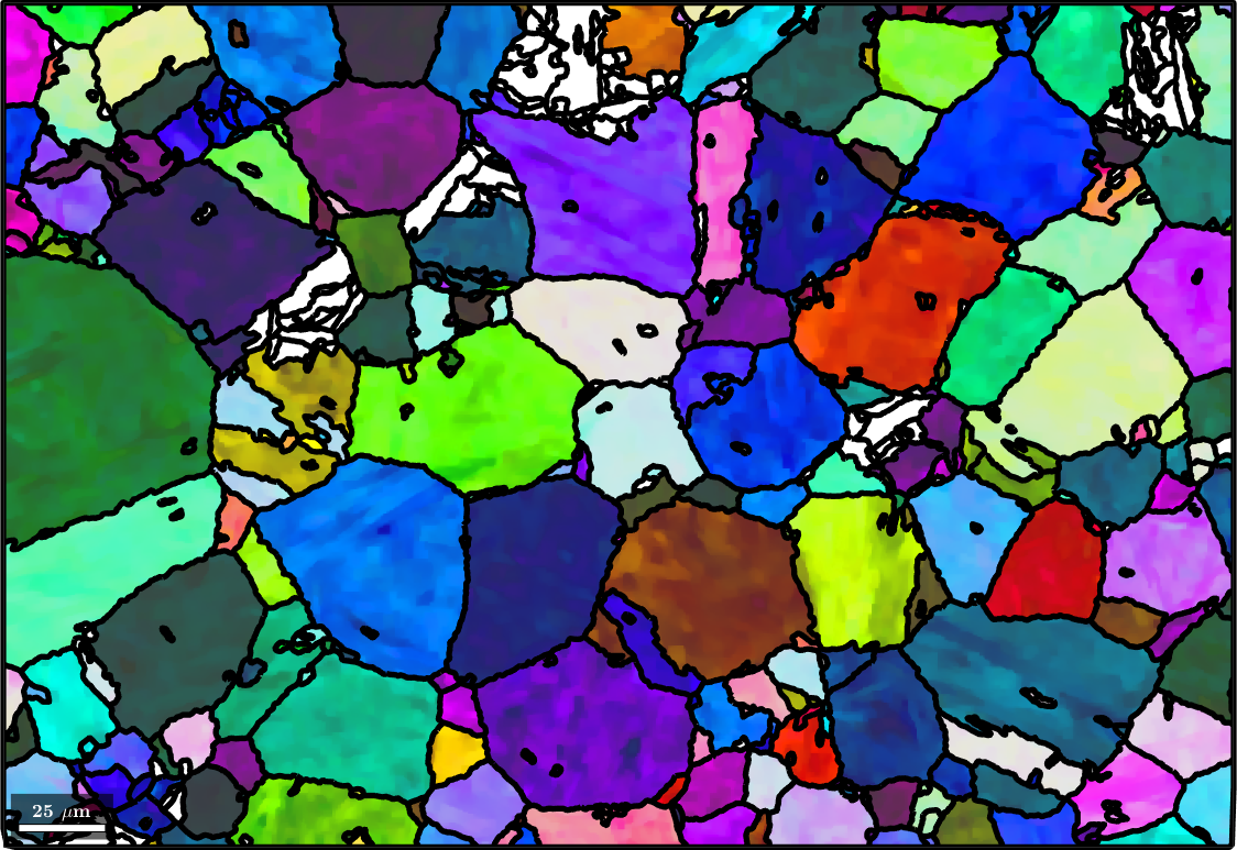
Summary of relevant thresholds
In the above script several parameters are decisive for the success of the reconstruction
- threshold for initial grain segmentation (3 degree)
- theshold (2 degree), tolerance (1.5 degree) and inflation power (p = 1.6) of the Markovian clustering algorithm
- maximum misfit within a parent grain (5 degree)
- minimum number of merged child grains
Triple Point Based Analysis
A problem of the boundary based reconstuction algorithm is that often child variants of different grains have a misorientation that is close to the theoretical child to child misorientation. One idea to overcome this problem is to analyze triple junctions. Now all three child orientations must fit to a common parent orientations. This fit is computed by the command calcParent.
% extract child orientations at triple junctions
tP = grains.triplePoints;
tPori = grains(tP.grainId).meanOrientation;

% compute the misfit to a common parent orientation
[~, fit] = calcParent(tPori,fcc2bcc,'id','threshold',5*degree);
Lets visualize this misfit by colorizing all triple junctions accordingly.
plot(ebsd('Iron bcc'),ebsd('Iron bcc').orientations,'figSize','large')
hold on
plot(grains.boundary,'linewidth',2)
hold off

hold on
plot(tP,fit(:,1) ./ degree,'MarkerEdgecolor','k','MarkerSize',8)
setColorRange([0,5])
mtexColorMap LaboTeX
mtexColorbar
hold off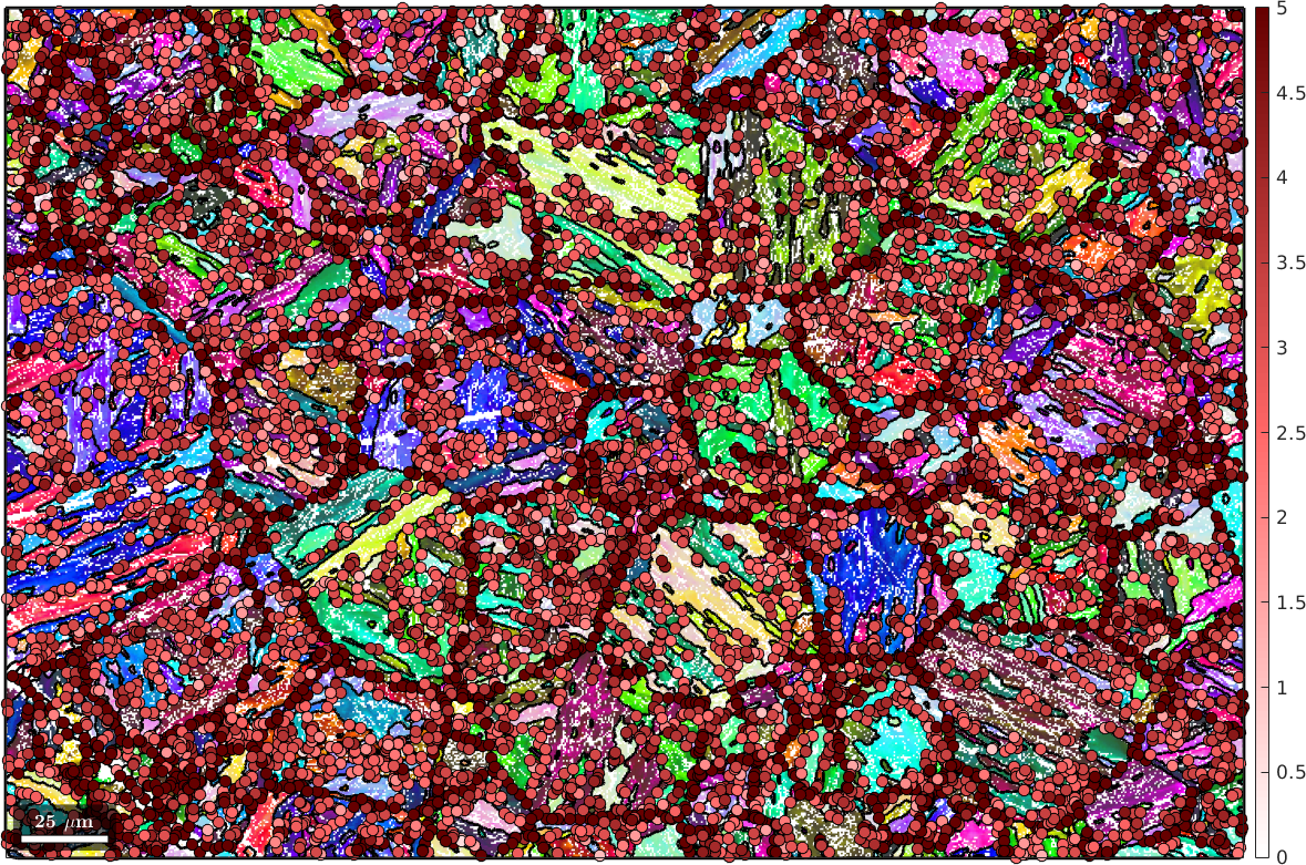
Again we observe, that triple junctions with large misfit outline the shape of the parent grains. In order to identify these parent grains we proceed analogously as for the boundary based analysis. We first set up a similarity matrix between grains connected to the same triple points and than use the Markovian clustering algorithm to detect clusters of child grains, which are than merged into parent grains.
Create a similarity matrix and reconstruct parent grains
The setup and the clustering of the similarity matrix is the same as above
threshold = 3*degree;
tol = 2*degree;

% compute the probabilities
prob = 1 - 0.5 * (1 + erf(2*(fit(:,1) - threshold)./tol));

% the corresponding similarity matrix
A = sparse(tP.grainId(:,1),tP.grainId(:,2),prob,length(grains),length(grains));
A = max(A, sparse(tP.grainId(:,2),tP.grainId(:,3),prob,length(grains),length(grains)));
A = max(A, sparse(tP.grainId(:,1),tP.grainId(:,3),prob,length(grains),length(grains)));

p = 1.4; % inflation power:
A = mclComponents(A,p);
Each connected component of the resulting adjacency matrix describes one parent grain. Hence, we can use this adjacency matrix to merge child grains into parent grains by the command merge.
% merge grains according to the adjacency matrix A
[parentGrains, parentId] = merge(grains,A);

% ensure grainId in parentEBSD is set up correctly with parentGrains
parentEBSD = ebsd;
parentEBSD('indexed').grainId = parentId(ebsd('indexed').grainId);
Let's visualize the result. Afterwards, we can proceed analogously as for the boundary based parent grain reconstruction described above.
plot(ebsd('Iron bcc'),ebsd('Iron bcc').orientations,'figSize','large')
hold on;
plot(parentGrains.boundary,'linewidth',4)
set(gcf,'Renderer','painters')
hold off