In this section, we discuss the austenite (fcc) to ferrite (bcc) phase transformation using an example EBSD data set of a Plessite microstructure from the Emsland iron meteorite. Plessite, from the Greek word "plythos" meaning "filling" iron, comprises an intimate mixed intergrowth of parent Taenite (austentic fcc) and child Kamacite (bcc). Plessite develops at low temperatures from retained Taenite and fills the spaces between Widmanstatten patterns. It occurs as the volumes remaining between already transformed Kamacite surrounded by very thin Taenite ribbons. Plessite contains child bcc and parent fcc phases, with the orientation of the fcc phase indicating the orientation of the formerly huge parent grains in the planetary body which can easily reach the dimension of meters.
% import the ebsd data
mtexdata emsland

% extract crystal symmetries
cs_bcc = ebsd('Fe').CS;
cs_aus = ebsd('Aus').CS;

% recover grains
[grains,ebsd.grainId] = calcGrains(ebsd('indexed'),'angle',5*degree,'minPixel',2);
grains = smooth(grains,4);
ebsd = EBSD (y↑→x)
Phase Orientations Mineral Color Symmetry Crystal reference frame
0 18393 (6.8%) notIndexed
1 215769 (80%) Ferrite, bcc LightSkyBlue m-3m
2 35838 (13%) Austenite DarkSeaGreen m-3m
Properties: bands, bc, bs, error, mad
Scan unit : um
X x Y x Z : [0, 604] x [0, 453] x [0, 0]
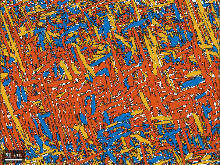
Normal vector: (0,0,1)The following lines plot bcc according to the crystallographic description of the selected reference direction (IPF coloring), whereas austenite is displayed as a phase in blue.
plot(ebsd('Fe'),ebsd('Fe').orientations)
hold on
plot(grains.boundary,'lineWidth',2,'lineColor','gray')
plot(grains('Aus'),'FaceColor','blue','DisplayName','Austenite')
hold off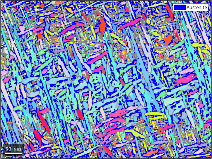
As expected, we recognize very small remaining fcc grains. This high-temperature phase is stabilized by the increasing nickel content during transformation. The low-temperature bcc phase can solve in maximum only 6\% nickel so that fcc has to assimilate the excess nickel. Size and amount of fcc is therefore and indication of the overall nickel content. Considering only the parent fcc phase, we display the orientations in an axis-angle plot.
plot(ebsd('Aus').orientations,'axisAngle')plot 2000 random orientations out of 32468 given orientations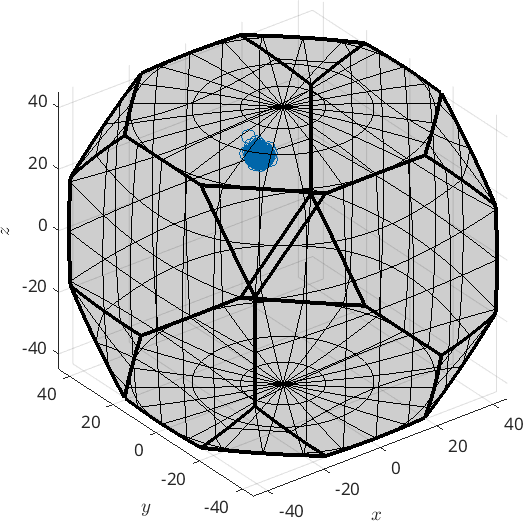
We recognize the uniform orientation of all fcc grains. Deviations are assumed to be the result of deformations during high-speed collisions in the asteroid belt. We can get this parent grain orientation by taking the mean and compute the fit by the command std
parenOri = mean(ebsd('Aus').orientations)

fit = std(ebsd('Aus').orientations) ./ degree
parenOri = orientation (Austenite → y↑→x)
Bunge Euler angles in degree
phi1 Phi phi2
266.294 163.623 245.508
fit =
1.4884Next, we display the bcc orientations (blue dots) in pole figures, and overlay the parent Taenite orientation (red dots) on top of them.
childOri = grains('Fe').meanOrientation;

h_bcc = Miller({1,0,0},{1,1,0},{1,1,1},cs_bcc);
h_fcc = Miller({1,0,0},{1,1,0},{1,1,1},cs_aus);

plotPDF(childOri,h_bcc,'MarkerSize',5,'MarkerFaceAlpha',0.05,'MarkerEdgeAlpha',0.1,'points',500);

nextAxis(1)
hold on
plot(parenOri * h_fcc(1).symmetrise ,'MarkerFaceColor','r')
xlabel('\((100)\)','Color','red','Interpreter','latex')

nextAxis(2)
plot(parenOri * h_fcc(3).symmetrise ,'MarkerFaceColor','r')
xlabel('\((111)\)','Color','red','Interpreter','latex')

nextAxis(3)
plot(parenOri * h_fcc(2).symmetrise ,'MarkerFaceColor','r')
xlabel('\((110)\)','Color','red','Interpreter','latex')
hold off

drawNow(gcm)
I'm plotting 500 random orientations out of 5248 given orientations
You can specify the the number points by the option "points".
The option "all" ensures that all data are plotted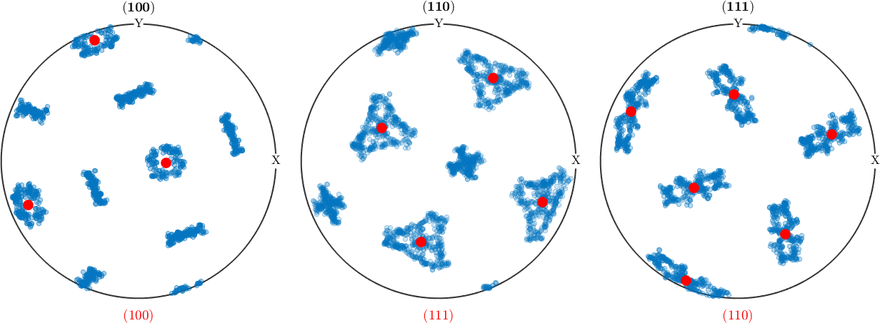
The partial coincidence of bcc and fcc poles suggests a crystallographic orientation relationship (OR) between both phases. The Kurdjumov-Sachs (KS) orientation relationship comprises a transition of one {111}-fcc plane into one {110}-bcc plane. Moreover, within these planes, one 110-fcc direction is parallel to one 111-bcc direction. For cubic crystals, identically indexed (hkl) and [uvw] generate the same directions. Thus, the derived pole figures can be used for both, the evaluation of directions as well as lattice plane normals.
While the MTEX command orientation.KurdjumovSachs(cs_aus,cs_bcc) could be used, let us define the orientation relationship explicitly:
KS = orientation.map(Miller(1,1,1,cs_aus),Miller(0,1,1,cs_bcc),...
Miller(-1,0,1,cs_aus),Miller(-1,-1,1,cs_bcc))
plotPDF(variants(KS,parenOri),'add2all','MarkerFaceColor','none','MarkerEdgeColor','k','linewidth',2)KS = misorientation (Austenite → Ferrite, bcc)
(111) || (011) [101̅] || [111̅]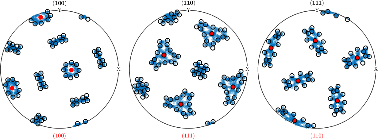
In order to quantify the match between the Kurdjumov-Sachs orientation relationship and the actual orientation relationship in the mapped plessitic area, we can compute the mean angular deviation between the ideal KS orientation relationship and all parent-to-child misorientations.
% Each parent-to-child misorientations can be calculated by
mori = inv(childOri) * parenOri;
% Whereas the mean angular deviation (output in degree) can be computed by
% the command
mean(angle(mori, KS)) ./ degree
%fit = sqrt(mean(min(angle_outer(childOri,variants(KS,parenOri)),[],2).^2))./degreeans =
3.9363Estimating the parent-to-child orientation relationship
We could ask ourselves if there is another orientation relationship that better matches the measured misorientations than the KS orientation relationship. In this case, a canonical candidate would be the mean of all misorientations.
% The mean of all measured parent-to-child misorientations:
p2cMean = mean(mori,'robust')
plotPDF(childOri,h_bcc,'MarkerSize',5,'MarkerFaceAlpha',0.05,'MarkerEdgeAlpha',0.1,'points',500);
hold on
plotPDF(variants(p2cMean,parenOri),'add2all','MarkerFaceColor','none','MarkerEdgeColor','k','linewidth',2)
hold off
% The mean angular deviation in degrees
mean(angle(mori, p2cMean)) ./ degreep2cMean = misorientation (Austenite → Ferrite, bcc)
Bunge Euler angles in degree
phi1 Phi phi2
198.978 8.19912 116.895
I'm plotting 500 random orientations out of 5248 given orientations
  You can specify the the number points by the option "points".
  The option "all" ensures that all data are plotted
ans =
2.4935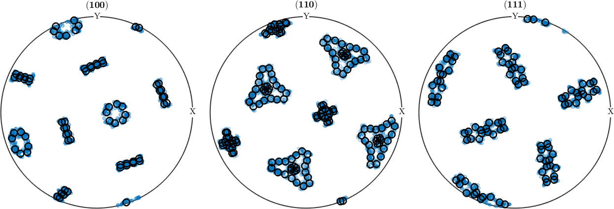
Here we make use of the fact that we know the parent orientation. If the parent orientation is entirely unknown, we may estimate the parent -to-child orientation relationship solely from child-to-child misorientations by the algorithm by Tuomo Nyyssönen and implemented in the function calcParent2Child. This iterative algorithm needs an orientation relationship not too far from the actual one as a starting point. Here we use the Nishiyama-Wassermann (NW) orientation relationship.
% Define the NW orientation relationship
NW = orientation.NishiyamaWassermann(cs_aus,cs_bcc)

% Extract all child to child misorientations
grainPairs = neighbors(grains('Fe'));
ori = grains(grainPairs).meanOrientation;

% Estimate a parent-to-child orientation relationship
p2cIter = calcParent2Child(ori,NW)

% The mean angular deviation
mean(angle(mori,p2cIter)) ./degree
NW = misorientation (Austenite → Ferrite, bcc)
(111) || (011) [11̅0] || [1̅00]
p2cIter = misorientation (Austenite → Ferrite, bcc)
Bunge Euler angles in degree
phi1 Phi phi2
177.427 98.0048 46.727
ans =
3.6950We observe that the parent-to-child orientation relationship computed solely from child-to-child misorientations fits the actual orientation relationship equally well.
Classification of child variants by variant Ids
Once we have determined parent orientations and a parent-to-child orientation relationship, we may proceed further by classifying the child orientations into different variants.
A variant refers to a specific orientation or crystallographic arrangement of the child phase within the context of the original parent orientation. Depending on the operative orientation relationship and parent-child crystal symmetries, a single parent phase orientation results in multiple child phase orientations (i.e.- variants). The variant Id is a convenient way to label or identify a specific variant within the child microstructure.
Child variant Ids are computed by the command calcVariantId.
% Compute for each child orientation a variantId
[variantId, packetId, bainId] = calcVariantId(parenOri,childOri,p2cIter,'morito');

% Colorize the orientations according to the variantID
color = ind2color(variantId,'ordered');
plotPDF(childOri,color,h_bcc,'MarkerSize',5);
I'm plotting 208 random orientations out of 5248 given orientations
You can specify the the number points by the option "points".
The option "all" ensures that all data are plotted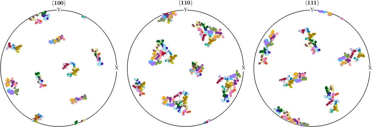
While it is very hard to distinguish the different variants in the pole figure plots, it becomes clearer in an axis angle plot
plot(childOri,color,'axisAngle')Warning: Setting the "WindowButtonDownFcn" property is not permitted while this
mode is active.
Warning: Setting the "WindowButtonUpFcn" property is not permitted while this
mode is active.
Warning: Setting the "KeyPressFcn" property is not permitted while this mode is
active.
Warning: Setting the "WindowScrollWheelFcn" property is not permitted while
this mode is active.
plot 2000 random orientations out of 5248 given orientations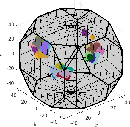
Classification of child variants by crystallographic packet Ids
An important classification is separating the variants into their various crystallographic packets.
A crystallographic packet Id is used to identify a packet of variants with the same habit plane (i.e. - the interfacial plane between the parent and child crystal lattices along which the atomic rearrangements occur during phase transformation).
Within a crystallographic packet, the individual variants are related to each other through specific symmetries. The crystallographic packet Id is a means of identifying and distinguishing a specific packet of variants that share the same habit plane and exhibit related crystallographic
A crystallographic packet Id is used to identify a packet of variants with the same habit plane (i.e. - the interfacial plane between the parent and child crystal lattices along which the atomic rearrangements occur during martensitic transformation).
Within a crystallographic packet, the individual variants are related to each other through specific symmetries. The crystallographic packet Id is a means of identifying and distinguishing a specific packet of variants that share the same habit plane and exhibit related crystallographic orientations.
color = ind2color(packetId);
plotPDF(childOri,color,h_bcc,'MarkerSize',5,'points',1000);

nextAxis(1)
hold on
opt = {'MarkerFaceColor','none','MarkerEdgeColor','k','linewidth',3};
plot(parenOri * h_fcc(1).symmetrise ,opt{:})
xlabel('\((100)\)','Color','red','Interpreter','latex')

nextAxis(2)
plot(parenOri * h_fcc(3).symmetrise ,opt{:})
xlabel('\((111)\)','Color','red','Interpreter','latex')

nextAxis(3)
plot(parenOri * h_fcc(2).symmetrise ,opt{:})
xlabel('\((110)\)','Color','red','Interpreter','latex')
hold off

drawNow(gcm)
I'm plotting 1000 random orientations out of 5248 given orientations
You can specify the the number points by the option "points".
The option "all" ensures that all data are plotted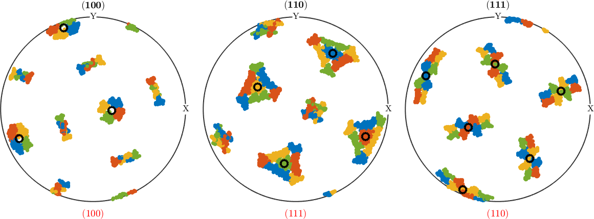
As we see from the above pole figures, the red, blue, orange and green orientations are distinguished by which of the symmetrically equivalent (111) austenite axes is aligned to the (110) ferrite axis.
We may also use the packet Id color to distinguish different child packets in the EBSD map.
plot(grains('Fe'),color)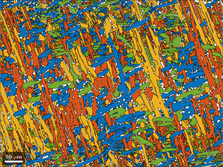
Classification of child variants by Bain group Ids
Another important classification is separating the variants into their various Bain groups.
The concept of Bain groups is based on the Bain notation.The latter provides a concise system of representing the transformation path and the geometric correspondence between the crystal structures of the parent and child phases. Each Bain group is labeled with a unique Bain group Id, which represents a distinct combination of orientation relationships between parent and child phases. Bain group Ids serve as a convenient identifier to categorize, classify and differentiate the various transformation paths that may occur during phase transformation based on their crystallographic characteristics.
The concept of Bain groups is based on the Bain notation.The latter provides a concise system of representing the transformation path and the geometric correspondence between the crystal structures of the parent austenite and child martensite phases. Each Bain group is labeled with a unique Bain group Id, which represents a distinct combination of orientation relationships between parent and child phases. Bain group Ids serve as a convenient identifier to categorize, classify and differentiate the various transformation paths that may occur during martensitic transformation based on their crystallographic characteristics.
color = ind2color(bainId);
plotPDF(childOri,color,h_bcc,'MarkerSize',5,'points',1000);

nextAxis(1)
hold on
opt = {'MarkerFaceColor','none','MarkerEdgeColor','k','linewidth',3};
plot(parenOri * h_fcc(1).symmetrise ,opt{:})
xlabel('\((100)\)','Color','red','Interpreter','latex')

nextAxis(2)
plot(parenOri * h_fcc(3).symmetrise ,opt{:})
xlabel('\((111)\)','Color','red','Interpreter','latex')

nextAxis(3)
plot(parenOri * h_fcc(2).symmetrise ,opt{:})
xlabel('\((110)\)','Color','red','Interpreter','latex')
hold off

drawNow(gcm)
I'm plotting 1000 random orientations out of 5248 given orientations
You can specify the the number points by the option "points".
The option "all" ensures that all data are plotted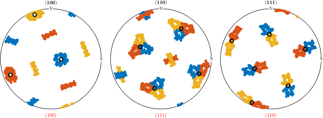
As we see from the above pole figures, the red, blue, and orange orientations are distinguished by which of the symmetrically equivalent (100) austenite axes is aligned to the (100) ferrite axis.
Similarly, we may also use the Bain group Id color to distinguish different child Bain groups in the EBSD map.
plot(grains('Fe'),color)