Inverse Pole Figure Color Coding of Orientation Maps

An orientation has three parameters and a colour has three numbers, so turning one into the other looks easy. It is not. Orientation space is curved and has crystal symmetry, whereas RGB colour space is a flat box. No map between them is simultaneously smooth, one to one, and free of arbitrary choices.

An inverse pole figure colour key is the usual compromise. It fixes one specimen direction and colours the crystal direction parallel to it. This page develops that construction, shows how to read the resulting map, and compares the keys used by MTEX and commercial EBSD systems.

The example assumes that the data has been imported and its reference frame has been checked. The basic map call is introduced in Plotting EBSD Maps. Inverse pole figures themselves are explained in Inverse Pole Figures.

plottingConvention.default('y↑→x');
mtexdata olivine silent
ebsd('olivine').CS = ebsd('olivine').CS.Laue;

From a crystal to a colour

Start with the crystal itself. Olivine grows with a characteristic habitus, which MTEX represents as a crystalShape.

cS = crystalShape.olivine;

plot(cS,'colored')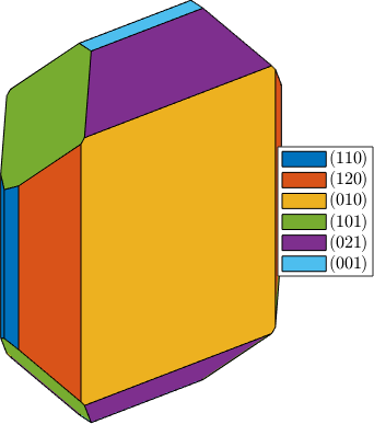

Opposite faces belong to the same symmetry-related face family. They therefore share one categorical colour. This plot is an analogy, not yet an IPF key: the colours distinguish faces but do not vary within a face.

The next plot places that shape in the measured mean orientation of each large grain. A grain is a phase-homogeneous, spatially connected region of EBSD measurements produced by segmentation. The reconstruction and boundary smoothing are explained in Grain Reconstruction.

% reconstruct the grains and attach their ids to the map
[grains,ebsd] = calcGrains(ebsd,'minPixel',5);

% smooth the pixel staircase of the grain boundaries
grains = smoothBoundary(grains,10);

% draw the boundaries and add crystals only to large grains
plot(grains.boundary,'lineWidth',1.5,'micronbar','off')
bigGrains = grains(grains.numPixel > 150);

hold on
plot(bigGrains('olivine'),0.8*cS,'lineWidth',2,'colored')
hold off
legend off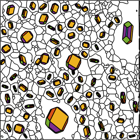

Seventy four grains are large enough to carry a crystal. Their different face directions make the orientation changes across the map visible. The idea of the colour key is to take the colour of the face that points towards you. A crystal shape has only six of them, so only six colours would ever appear. A continuous key replaces the faceted crystal by a ball whose surface colour varies continuously.

close all;
ipfKey = ipfHSVKey(ebsd('olivine'));
plot(ipfKey,'3d')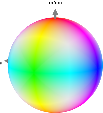

The coloured sphere is the continuous counterpart of the crystal shape. Red, green, and blue anchor specific crystal directions, and the colours between them vary smoothly.

Placing one sphere on each large grain and turning it by the grain's mean orientation connects the key back to the map.

plot(grains.boundary,'lineWidth',1.5,'micronbar','off')

hold on
plot(bigGrains('olivine'),ipfKey)
hold off
legend off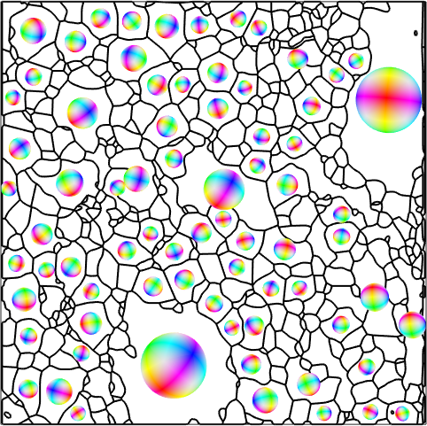

Each sphere is turned differently, but its point facing the viewer is the point that matters. Its colour becomes the single colour of that grain.

colors = ipfKey.orientation2color(bigGrains('olivine').meanOrientation);
plot(bigGrains('olivine'),colors)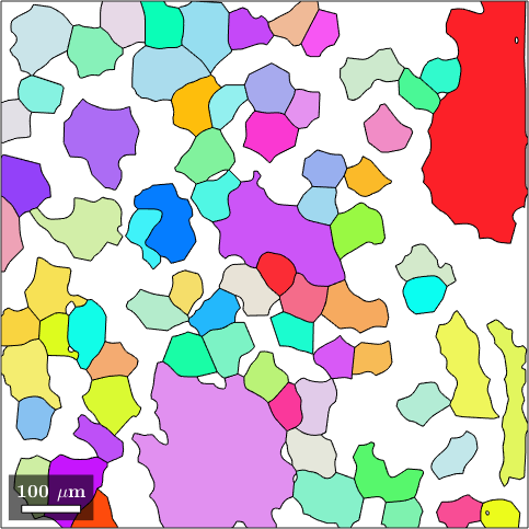

The grain colours now reproduce the centres of the spheres in the preceding figure. The geometry has disappeared, but the selected crystal direction has been retained as colour.

Reading the map

Flattening the coloured sphere into a stereographic projection turns it into the legend for the map.

plot(ipfKey,'complete','upper')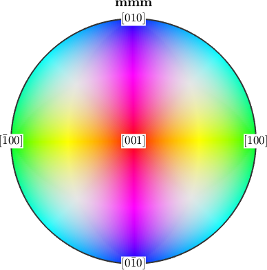

The option 'complete' draws the whole upper hemisphere, with \([001]\) in the centre, \([100]\) at both ends of the horizontal, and \([010]\) at top and bottom. Orthorhombic symmetry makes the four quadrants repeat the same colours mirrored, so one quadrant already carries every colour the key can produce. That quadrant is the fundamental sector, which holds one symmetry-equivalent representative of every crystal direction, and the key normally plots only it.

For this olivine setting, red means that the crystal \(c\) axis is parallel to the specimen normal. Green represents the \(a\) axis and blue the \(b\) axis. Intermediate directions receive intermediate colours.

The same information can be plotted in the inverse pole figure itself. Each grain is placed at the crystal direction parallel to the normal, and marker area is scaled by grain area.

plotIPDF(bigGrains('olivine').meanOrientation,colors,vector3d.Z,...
  'MarkerSize',0.05*bigGrains('olivine').area,'markerEdgeColor','k')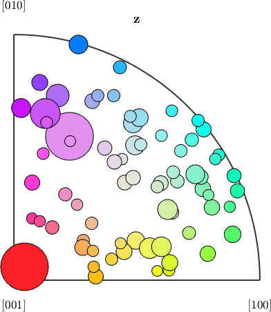

The markers cover the sector rather than clustering in one corner. These large grains therefore have no single strongly preferred crystal axis along the specimen normal. Two markers stand out by size: the red one in the \([001]\) corner, 6 degrees from the \(c\) axis, and the pale magenta one in the interior, 53 degrees from it. Their grain areas are within one percent of each other, so the two largest grains of this map sit at quite different crystal directions.

An IPF map does not retain a complete orientation. It records where one specimen direction falls in the crystal frame and discards the remaining rotation about that direction. Equal colours therefore do not prove that two orientations are equal.

Choosing the reference direction

Nothing forces the fixed direction to be the specimen normal. It may be a rolling direction, a foliation, or the axis of a cylindrical specimen. The property that stores this choice is ipfDirection.

% colour the map by the specimen x direction
ipfKey.ipfDirection = vector3d.X;
colors = ipfKey.orientation2color(ebsd('olivine').orientations);
plot(ebsd('olivine'),colors)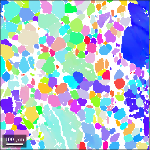

The microstructure is unchanged, but the colours are completely different. Before comparing two IPF maps, check that they use the same phase symmetry, specimen reference direction, and colour-key algorithm. Also check the specimen reference frame: an incorrect frame produces a plausible map with incorrect colours.

The ipfDirection may also be a list with one direction per measurement. This is useful for a curved specimen, where the local surface normal changes across the map.

Customizing the color key

Colour placement within the sector is conventional. It can be moved without changing which crystal directions the key distinguishes. Reflecting the colour space interchanges green and blue.

ipfKey.colorPostRotation = reflection(yvector);
plot(ipfKey)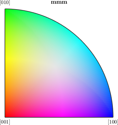

The sector has the same shape and the same white centre, but its green and blue corners have exchanged places. Rotating the colour space by 120° instead cycles red, green, and blue.

ipfKey.colorPostRotation = rotation.byAxisAngle(zvector,120*degree);
plot(ipfKey)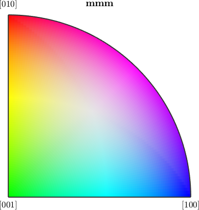

Again only the colour assignment has moved. The crystal symmetry, reference direction, and orientations have not changed.

Laue or enantiomorphic symmetry groups

The example began by assigning the olivine phase its Laue group, mmm. This identifies crystal directions related by the improper operations in that group. A key can instead use the proper subgroup, 222, whose operations are rotations only.

EBSD systems report orientations as Euler angles, and Euler angles describe proper rotations. This does not mean that an EBSD pattern can never contain information about polarity. The symmetry used to index the pattern and the symmetry used to reduce directions for colouring are choices that must be stated separately.

% use only the proper rotations of the olivine point group
ipfKey = ipfHSVKey(ebsd('olivine').CS.properGroup);
plot(ipfKey)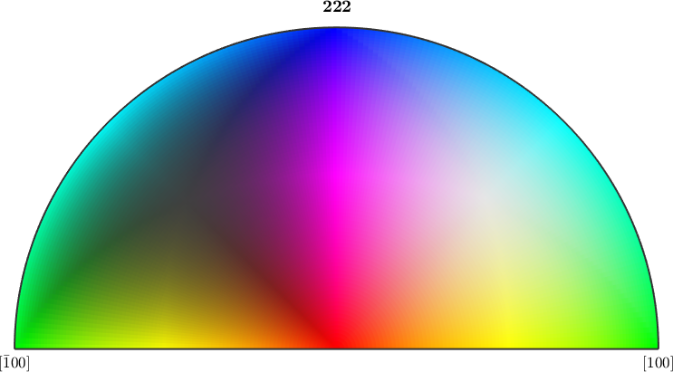

The 222 group has half as many operations as mmm. Its fundamental sector is therefore twice as large: half of the upper hemisphere rather than one quarter. The extra area distinguishes directions that the Laue key assigned the same colour.

close all;
colors = ipfKey.orientation2color(ebsd('olivine').orientations);
plot(ebsd('olivine'),colors)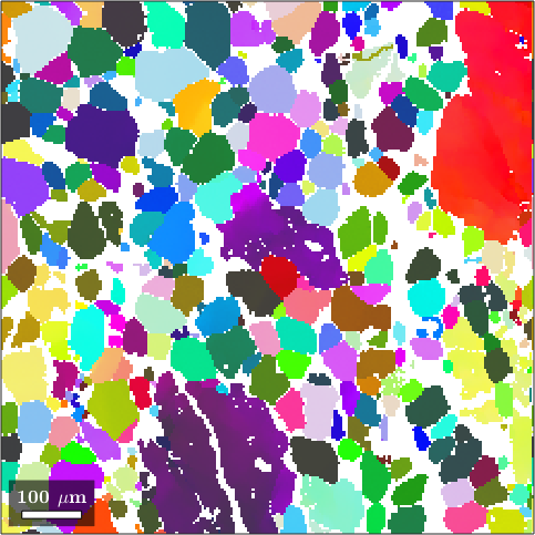

The proper-group map contains colour distinctions that the earlier Laue map suppressed. This is additional displayed information only if 222 is the symmetry intended for the analysis; it is not a sharper rendering of the same equivalence relation.

Other inverse pole figure keys

Commercial EBSD systems use different colour assignments. MTEX provides TSL/OIM and HKL Channel 5 keys so that their maps can be reproduced. These two constructors use the Laue group of the supplied phase.

plot(ipfTSLKey(ebsd('olivine').CS))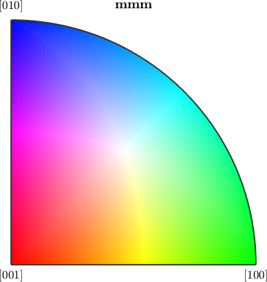

For orthorhombic olivine, the TSL key is difficult to distinguish from the default MTEX key. Its centre remains bright and the three crystal axes retain the familiar corner colours.

plot(ipfHKLKey(ebsd('olivine').CS))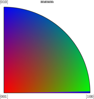

The HKL key blends the three corner colours directly. Its sector becomes dark in the middle, whereas the MTEX and TSL keys keep a bright centre.

A more serious difference appears for symmetry groups whose sector cannot be mapped smoothly and one to one onto the colour box. A discontinuous key gives different colours to directions only a fraction of a degree apart. The resulting map can contain a colour edge that is not a grain boundary. MTEX prints a warning when such a key is constructed.

plot(ipfTSLKey(crystalSymmetry('-3m')),'complete','upper')

Warning: The point group "-3m1" has no topologically correct color key: its
         fundamental sector cannot be mapped smoothly and one to one onto the
         color space, so the colors jump somewhere. Expect it between green and
         blue.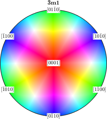

The warning is intentional, but the drawn hemisphere looks perfectly smooth: neighbouring directions 0.05 degrees apart differ by at most 0.003 in RGB. The jump is not inside the disc, it is on its rim. Plot the other hemisphere and compare the two rims.

plot(ipfTSLKey(crystalSymmetry('-3m')),'complete','lower')

Warning: The point group "-3m1" has no topologically correct color key: its
         fundamental sector cannot be mapped smoothly and one to one onto the
         color space, so the colors jump somewhere. Expect it between green and
         blue.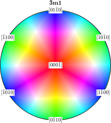

At \([01\bar{1}0]\) the upper hemisphere ends in green and the lower one begins in blue, and over 91 percent of the rim the two sides differ by more than 0.1 in RGB. A crystal direction that lies almost in the specimen plane can therefore change colour completely under a fraction of a degree of measurement noise. The resulting colour edge in a map is a property of the key, not evidence of a physical boundary.

The maths behind an IPF colour

Let the orientation \(\mathbf{O}\) map crystal coordinates into specimen coordinates, and let \(\mathbf{r}\) be the fixed specimen direction. The inverse pole figure direction in crystal coordinates is

\[ \mathbf{h} = \mathbf{O}^{-1}\mathbf{r}. \]

Crystal symmetry maps \(\mathbf{h}\) to one representative in the fundamental sector. The direction key then maps that representative to an RGB triplet. Because many orientations can produce the same \(\mathbf{h}\), this construction cannot be one to one in orientation space.

Further reading

Next

Orientation Plots shows the same measurements as pole figures, inverse pole figures, and sections through orientation space. Sharp Color Keys increases contrast when a phase occupies only a small orientation range. Advanced Color Keys covers Euler-angle, axis-angle, and spot keys.