Radial Basis Functions on SO(3)

Radial Basis Functions on SO(3) edit page

In MTEX we describe radial basis functions on the rotation group \(SO(3)\) by the class SO3FunRBF.

This includes the following three types of ODFs.

The Uniform ODF

The uniform ODF

\[f(g) = 1,\quad g \in SO(3),\]

is everywhere identical to one. In order to define a uniform ODF one needs only to specify its crystal and specimen symmetry and to use the command uniformODF.

cs = crystalSymmetry('cubic');
ss = specimenSymmetry('orthorhombic');
odf = uniformODF(cs,ss)

odf = SO3FunRBF (m-3m → xyz (mmm))
 
  uniform component
  weight: 1

Unimodal ODFs

An unimodal ODF

\[f(g; x) = \psi (\angle(g,x)),\quad g \in SO(3),\]

is specified by a radial symmetrical function \(\psi\) centered at a modal orientation, \(x\in SO(3)\). In order to define a unimodal ODF one needs

a preferred orientation mod1
a kernel function psi defining the shape
the crystal symmetry

cs = crystalSymmetry('432');
ori = orientation.byMiller([1,2,2],[2,2,1],cs);
psi = SO3vonMisesFisherKernel('halfwidth',10*degree);
odf1 = unimodalODF(ori,psi)

plotPDF(odf1,[Miller(1,0,0,cs),Miller(1,1,0,cs)],'antipodal')

odf1 = SO3FunRBF (432 → xyz)
 
  unimodal component
  kernel: van Mises Fisher, halfwidth 10°
  center: 1 orientations
 
  Bunge Euler angles in degree
     phi1     Phi    phi2  weight
  116.565 48.1897 26.5651       1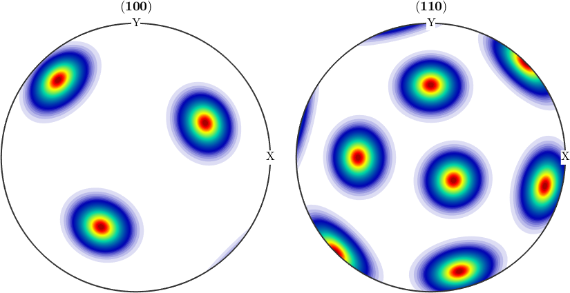

For simplicity one can also omit the kernel function. In this case the default SO(3) de la Vallee Poussin kernel is chosen with half width of 10 degree.

Multimodal ODFs

We define a second unimodal ODF with same kernel function and same crystal symmetry at an other orientation.

ori2 = orientation.byMiller([1,1,2],[0,2,1],cs)
odf2 = unimodalODF(ori2,psi)

plotPDF(odf2,[Miller(1,0,0,cs),Miller(1,1,0,cs)],'antipodal')

ori2 = orientation (432 → xyz)
 
  Bunge Euler angles in degree
     phi1     Phi    phi2
  309.232 35.2644      45
 
 
odf2 = SO3FunRBF (432 → xyz)
 
  unimodal component
  kernel: van Mises Fisher, halfwidth 10°
  center: 1 orientations
 
  Bunge Euler angles in degree
     phi1     Phi    phi2  weight
  309.232 35.2644      45       1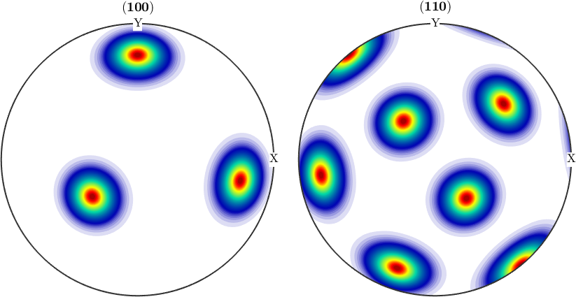

By adding this unimodal ODFs we get an so called multimodal ODF, which by construction is the sum of the radial symmetrical function \(\psi\) centered at some orientations.

odf3 = odf1 + odf2

plotPDF(odf3,[Miller(1,0,0,cs),Miller(1,1,0,cs)],'antipodal')

odf3 = SO3FunRBF (432 → xyz)
 
  multimodal components
  kernel: van Mises Fisher, halfwidth 10°
  center: 2 orientations
 
  Bunge Euler angles in degree
     phi1     Phi    phi2  weight
  116.565 48.1897 26.5651       1
  309.232 35.2644      45       1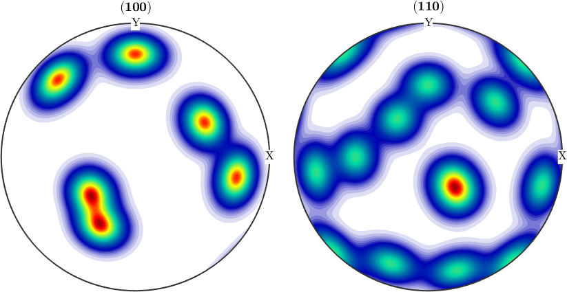

Its also possible to define an multimodal ODF by more than two orientations, for example

odf4 = SO3FunRBF.example

plotPDF(odf4,[Miller(1,0,0,odf4.CS),Miller(1,1,0,odf4.CS)],'antipodal')

odf4 = SO3FunRBF (-3m1 → xyz)
 
  multimodal components
  kernel: de la Vallee Poussin, halfwidth 5°
  center: 19848 orientations, resolution: 5°
  weight: 1