Low Level Parent Phase Reconstruction

Low Level Parent Phase Reconstruction edit page

In this section we discuss parent grain reconstruction at the example of a titanium alloy. Lets start by importing a sample data set

mtexdata alphaBetaTitanium

% the phase names for the alpha and beta phases
alphaName = 'Ti (alpha)';
betaName = 'Ti (Beta)';

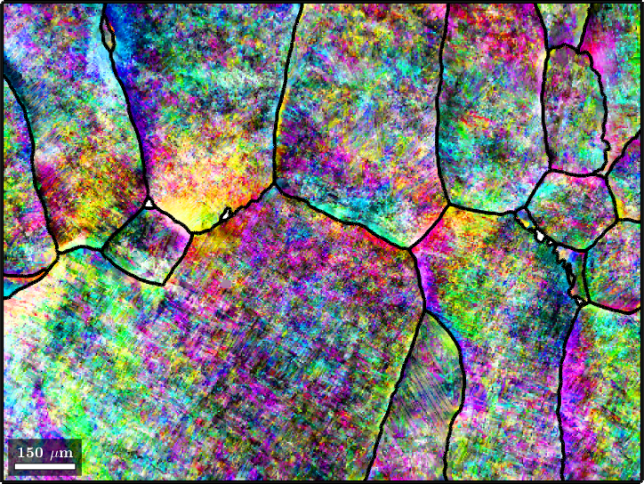
% and plot the alpha phase as an inverse pole figure map
plot(ebsd(alphaName),ebsd(alphaName).orientations,'figSize','large')

saving data to /home/hielscher/mtex/master/data/alphabetatitanium.mat
 
ebsd = EBSD
 
 Phase  Orientations     Mineral         Color  Symmetry  Crystal reference frame
     0  10449 (5.3%)  notIndexed                                                 
     1   437 (0.22%)   Ti (BETA)  LightSkyBlue       432                         
     2  185722 (94%)  Ti (alpha)  DarkSeaGreen       622       X||a*, Y||b, Z||c*
 
 Properties: bands, bc, bs, error, mad, reliabilityindex, x, y
 Scan unit : um

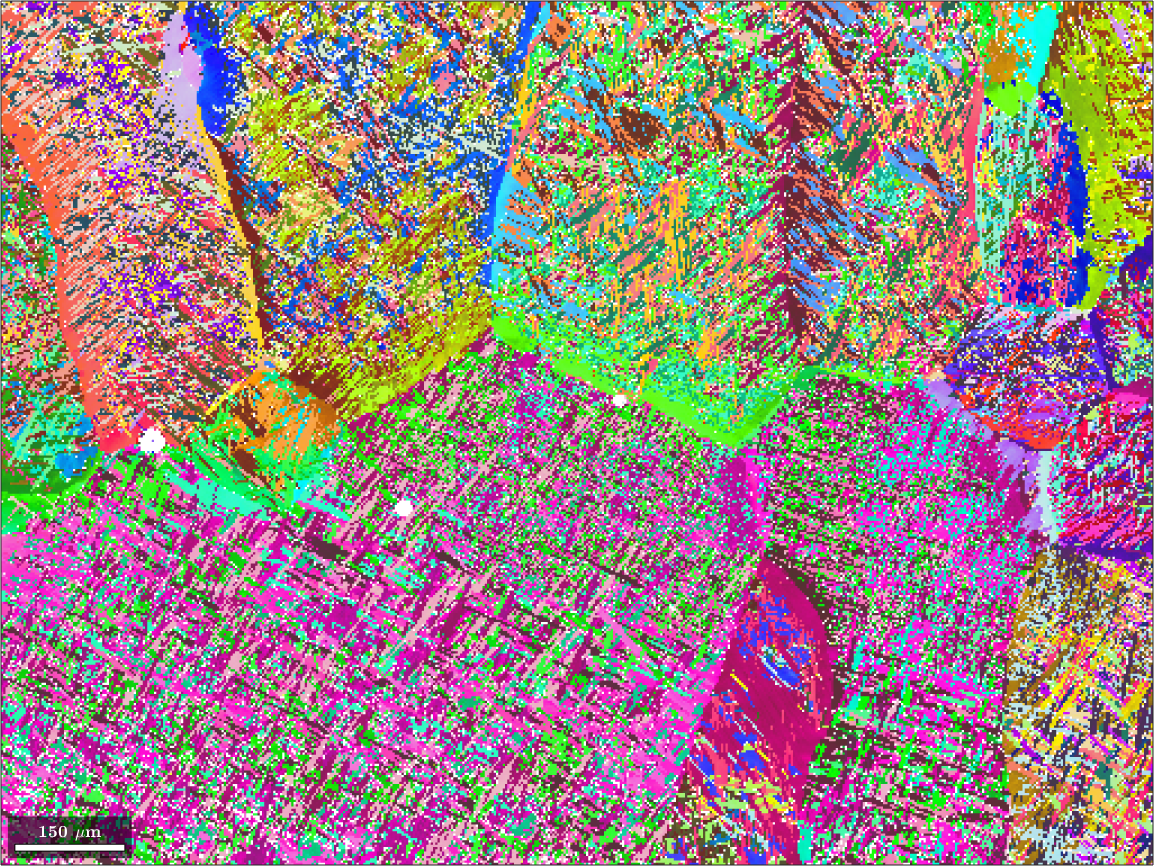
The data set contains 99.8 percent alpha titanium and 0.2 percent beta titanium. Our goal is to reconstuct the original beta phase. The original grain structure appears almost visible for human eyes. Our computations will be based on the Burgers orientation relationship

beta2alpha = orientation.Burgers(ebsd(betaName).CS,ebsd(alphaName).CS)

beta2alpha = misorientation (Ti (BETA) → Ti (alpha))
 
 (110) || (0001)   [1-11] || [-2110]

that alligns (110) plane of the beta phase with the (0001) plane of the alpha phase and the [1-11] direction of the beta phase with the [2110] direction of the alpha phase.

Note that all MTEX functions for parent grain reconstruction expect the orientation relationship as parent to child and not as child to parent.

Detecting triple points that belong to the same parent orientation

In a first step we want to identify triple junctions that have misorientations that are compatible with a common parent orientations. To this end we first compute alpha grains using the option removeQuadruplePoints which turn all quadruple junctions into 2 triple junctions. Furthermore, we choose a very small threshold of 1.5 degree for the identification of grain boundaries to avoid alpha orientations that belong to different beta grains get merged into the same alpha grain.

% reconstruct grains
[grains,ebsd.grainId] = calcGrains(ebsd('indexed'),'threshold',1.5*degree,...
  'removeQuadruplePoints');
grains = smooth(grains,1,'moveTriplePoints');

% plot all alpha pixels
region = [299 401 -500 -440];
plot(ebsd(alphaName),ebsd(alphaName).orientations,...
  'region',region,'micronbar','off','figSize','large');

% and on top the grain boundaries
hold on
plot(grains.boundary,'linewidth',2 ,'region',region);
hold off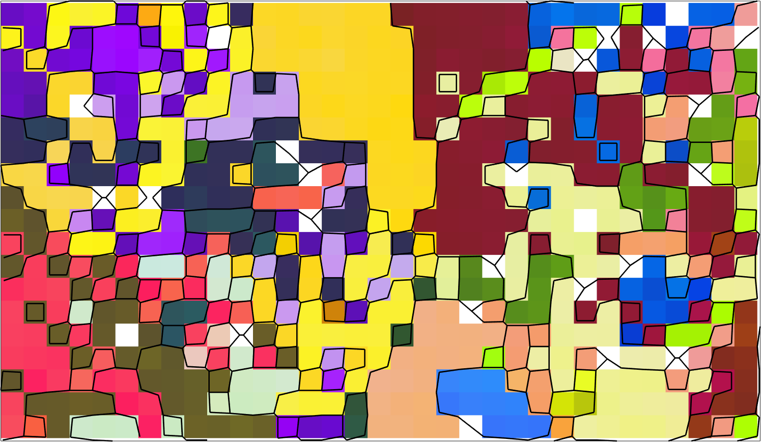

Above we have plotted only a very small subregion of the original data set to make the seperation of the qudruple junctions better visible.

Next we extract all alpha - alpha - alpha triple junctions and use the command calcParent to find for each of these triple junctions the best fitting parent orientations.

% extract all alpha - alpha - alpha triple points
tP = grains.triplePoints(alphaName,alphaName,alphaName)

% compute for each triple point the best fitting parentId and how well the fit is
tPori = grains(tP.grainId).meanOrientation;
[parentId, fit] = calcParent(tPori,beta2alpha,'numFit',2,'id','threshold',5*degree);

tP = triplePointList
 
 points   mineral 1   mineral 2   mineral 3
  93759  Ti (alpha)  Ti (alpha)  Ti (alpha)

The command calcParent returns for each child orientation a parentId which allows us later to compute the parent orientation from the child orientation. Furthermore, the command return for each triple junction the misfit between the adjecent parent orientations in radiant. Finally, the option 'numFit',2 causes calcParent to return not only the best fit but also the second best fit. This will be used later. First we simple colorize the triple junctions according to the best fit.

hold on
plot(tP,fit(:,1) ./ degree,'MarkerEdgecolor','k','MarkerSize',10,'region',region)
setColorRange([0,5])
mtexColorMap LaboTeX
mtexColorbar
hold off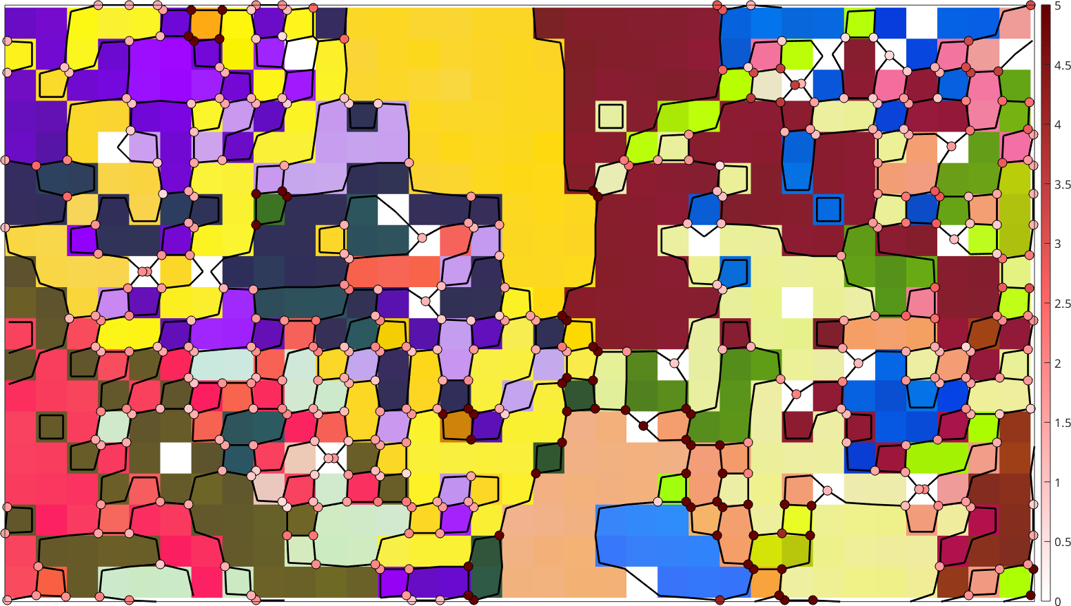

Next we select those triple junctions as reliable that have a fit less than 2.5 degree and second best fit that is larger than 2.5 degree

consistenTP = fit(:,1) < 2.5*degree & fit(:,2) > 2.5*degree;

% marke these triple points by a red cicle
hold on
plot(tP(consistenTP),'MarkerEdgecolor','r','MarkerSize',10,...
  'MarkerFaceColor','none','linewidth',2,'region',region)
hold off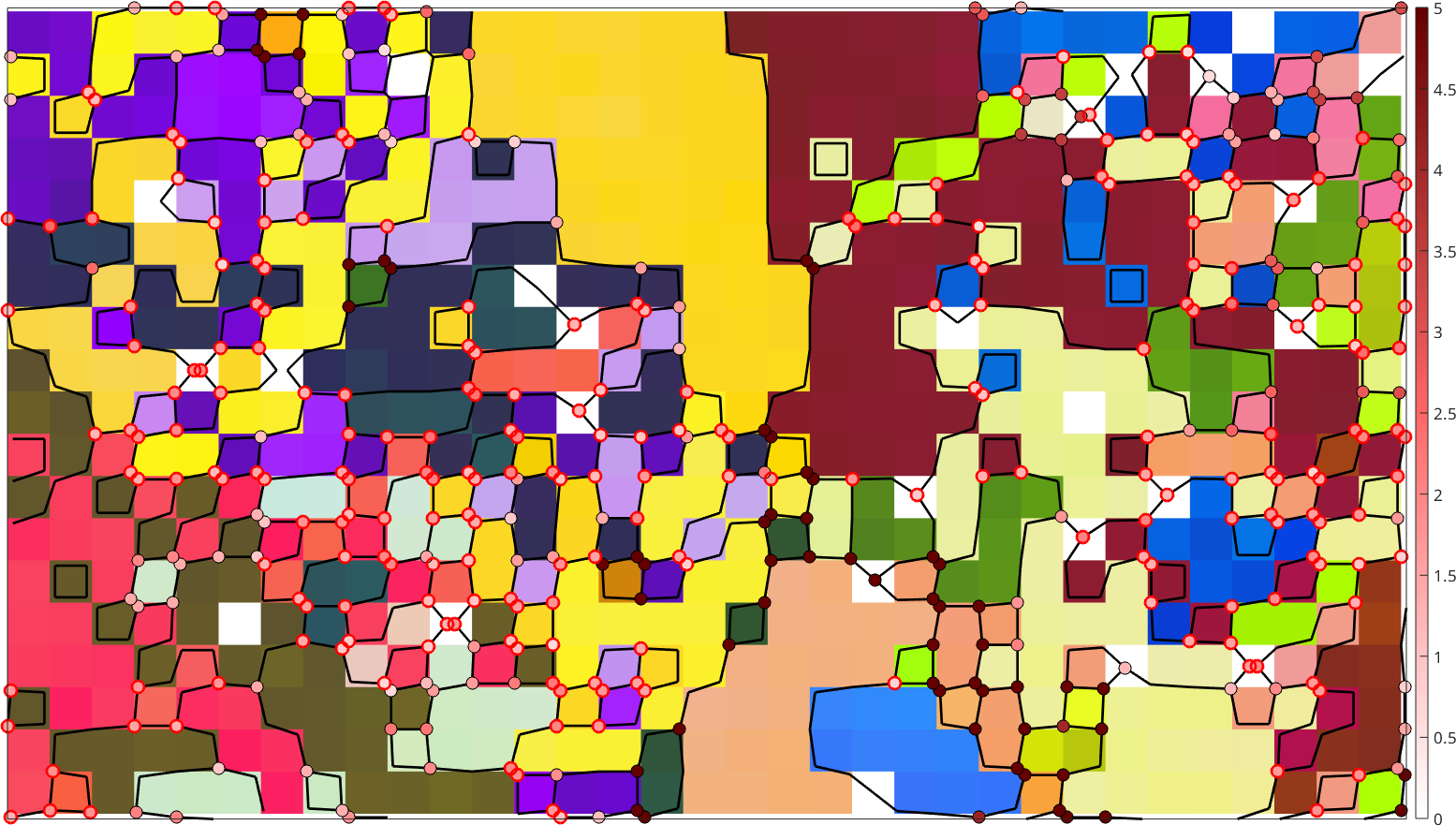

Recover beta grains from consistent triple junctions

We observe that despite the quite sharp threshold we have many consistent triple points. In the next step we check wether all consistent triple junctions of a grain vote for the same parent orientation. Such a check for consistent votes can be computed by the command majorityVote using the option strict.

% get a unique parentId vote for each grain
[parentId, numVotes] = majorityVote( tP(consistenTP).grainId, ...
  parentId(consistenTP,:,1), max(grains.id),'strict');

The command majorityVote returns for each grain with consistent parentId votes this unique parentId and for all other grains NaN. The second output argument gives the number of these votes

For all grains with at least 3 unique vote we now use the command variants to compute the parent orientation corresponding to the parentId. This parent orientations we assign as new meanOrientation to our grains.

% lets store the parent grains into a new variable
parentGrains = grains;

% change orientations of consistent grains from child to parent
parentGrains(numVotes>2).meanOrientation = ...
  variants(beta2alpha,grains(numVotes>2).meanOrientation,parentId(numVotes>2));

% update all grain properties that are related to the mean orientation
parentGrains = parentGrains.update;

Lets plot map of these reconstructed beta grains

% define a color key
ipfKey = ipfColorKey(ebsd(betaName));
ipfKey.inversePoleFigureDirection = vector3d.Y;

% and plot
plot(parentGrains(betaName), ...
  ipfKey.orientation2color(parentGrains(betaName).meanOrientation),'figSize','large')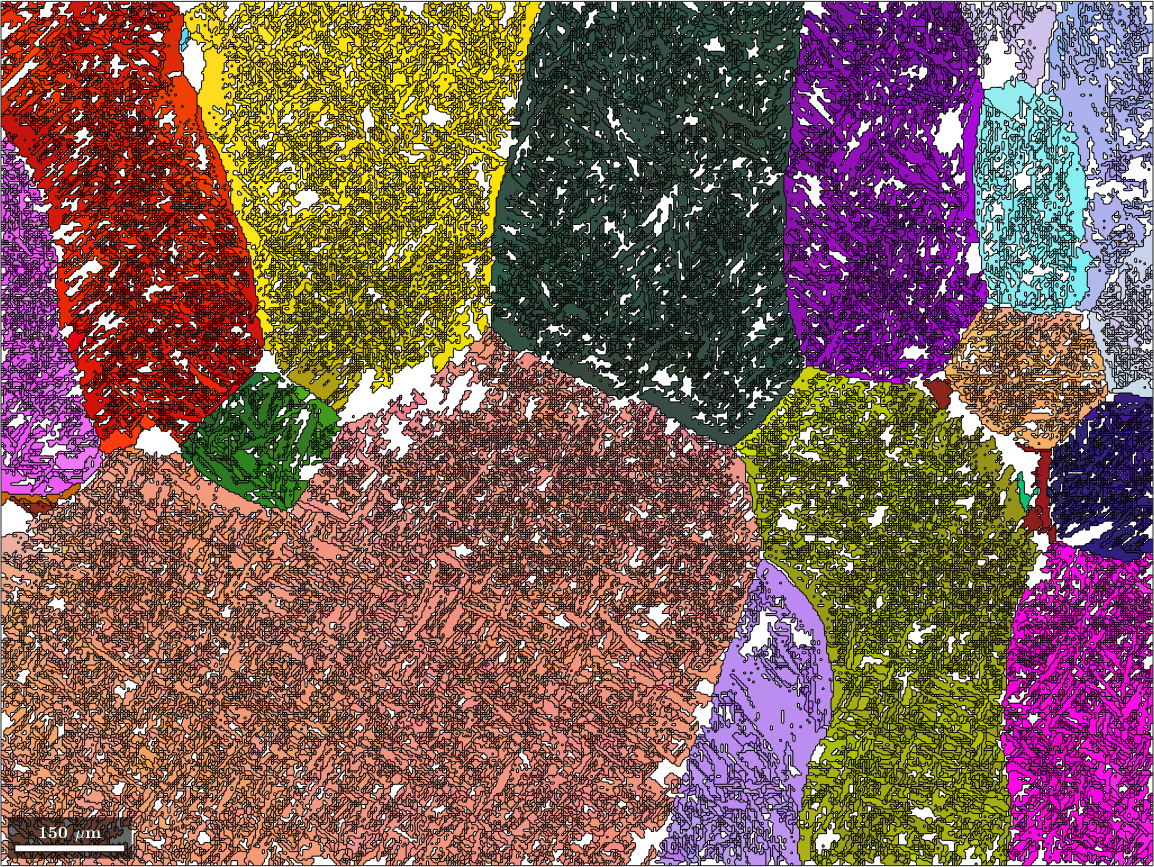

We observe that this first step already results in very many Beta grains. However, the grain boundaries are still the boundaries of the original alpha grains. To overcome this, we merge all Beta grains that have a misorientation angle smaller then 2.5 degree.

As an additional consistency check we verify that each parent grain has been reconstructed from at least 2 child grains. To this end we first make a testrun the merge operation and then revert all parent grains that that have less then two childs. This step may not nessesary in many case.

% test run of the merge operation
[~,parentId] = merge(parentGrains,'threshold',2.5*degree,'testRun');

% count the number of neighbouring child that would get merged with each child
counts = accumarray(parentId,1);

% revert all beta grains back to alpha grains if they would get merged with
% less then 1 other child grains
setBack = counts(parentId) < 2 & grains.phaseId == grains.name2id(alphaName);
parentGrains(setBack).meanOrientation = grains(setBack).meanOrientation;
parentGrains = parentGrains.update;

Now we perform the actual merge and the reconstruction of the parent grain boundaries.

% merge beta grains
[parentGrains,parentId] = merge(parentGrains,'threshold',2.5*degree);

% set up a EBSD map for the parent phase
parentEBSD = ebsd;

% and store there the grainIds of the parent grains
parentEBSD('indexed').grainId = parentId(ebsd('indexed').grainId);

plot(parentGrains(betaName), ...
  ipfKey.orientation2color(parentGrains(betaName).meanOrientation),'figSize','large')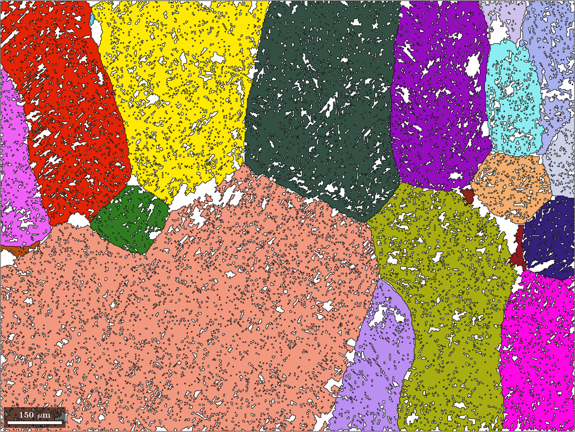

Merge alpha grains to beta grains

After the first two steps we have quite some alpha grains have not yet transformed into beta grains. In order to merge those left over alpha grains we check whether their misorientation with one of the neighbouring beta grains coincides with the parent to grain orientation relationship and if yes merge them evantually with the already reconstructed beta grains.

First extract a list of all neighbouring alpha - beta grains

% all neighbouring alpha - beta grains
grainPairs = neighbors(parentGrains(alphaName), parentGrains(betaName));

and check how well they fit to a common parent orientation

% extract the corresponding meanorientations
oriAlpha = parentGrains( grainPairs(:,1) ).meanOrientation;
oriBeta = parentGrains( grainPairs(:,2) ).meanOrientation;

% compute for each alpha / beta pair of grains the best fitting parentId
[parentId, fit] = calcParent(oriAlpha,oriBeta,beta2alpha,'numFit',2,'id');

Similarly, as in the first step the command calcParent returns a list of parentId that allows the convert the child orientations into parent orientations using the command variants and the fitting to the given parent orientation. Similarly, as for the triple point we select only those alpha beta pairs such that the fit is below the threshold of 2.5 degree and at the same time the second best fit is above 2.5 degree.

% consistent pairs are those with a very small misfit
consistenPairs = fit(:,1) < 5*degree & fit(:,2) > 5*degree;

Next we compute for all alpha grains the majority vote of the surounding beta grains and change their orientation from alpha to beta

parentId = majorityVote( grainPairs(consistenPairs,1), ...
  parentId(consistenPairs,1), max(parentGrains.id));

% change grains from child to parent
hasVote = ~isnan(parentId);
parentGrains(hasVote).meanOrientation = ...
  variants(beta2alpha, parentGrains(hasVote).meanOrientation, parentId(hasVote));

% update grain boundaries
parentGrains = parentGrains.update;

% merge new beta grains into the old beta grains
[parentGrains,parentId] = merge(parentGrains,'threshold',5*degree);

% update grainId in the ebsd map
parentEBSD('indexed').grainId = parentId(parentEBSD('indexed').grainId);

% plot the result
color = ipfKey.orientation2color(parentGrains(betaName).meanOrientation);
plot(parentGrains(betaName),color,'linewidth',2)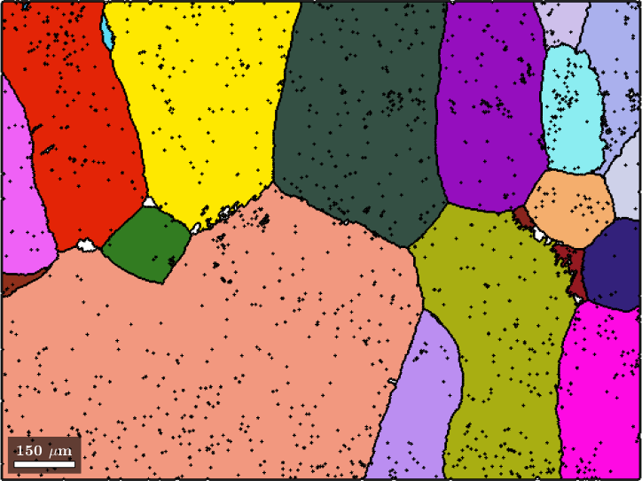

The above step has merged

sum(hasVote)

ans =
       15535

alpha grains into the already reconstructed beta grain. This reduces the amount of grains not yet reconstructed to

sum(parentGrains('Ti (alpha').grainSize) ./ sum(parentGrains.grainSize)*100

ans =
    1.2253

percent. One way to proceed would be to repeat the steps of this section multiple time, maybe with increasing threshold, until the percentage of reconstructed beta grains is sufficiently high. Another approach in to consider the left over alpha grains as noise and use denoising techniques to replace them with beta orientations. This will be done in the last section.

Reconstruct beta orientations in EBSD map

Until now we have only recovered the beta orientations as the mean orientations of the beta grains. In this section we want to set up the EBSD variable parentEBSD to contain for each pixel a reconstruction of the parent phase orientation.

Therefore, we first identify all pixels that previously have been alpha titanium but now belong to a beta grain.

% consider only original alpha pixels that now belong to beta grains

isNowBeta = parentGrains.phaseId(max(1,parentEBSD.grainId)) == ebsd.name2id(betaName) &...
  parentEBSD.phaseId == ebsd.name2id(alphaName);

Next we can use once again the function calcParent to recover the original beta orientation from the measured alpha orientation giving the mean beta orientation of the grain.

% update beta orientation
[parentEBSD(isNowBeta).orientations, fit] = calcParent(parentEBSD(isNowBeta).orientations,...
  parentGrains(parentEBSD(isNowBeta).grainId).meanOrientation,beta2alpha);

We obtain even a measure fit for the corespondence between the beta orientation reconstructed for a single pixel and the beta orientation of the grain. Lets visualize this measure of fit

% the beta phase
plot(parentEBSD(isNowBeta),fit ./ degree,'figSize','large')
mtexColorbar
setColorRange([0,5])
mtexColorMap('LaboTeX')

hold on
plot(parentGrains.boundary,'lineWidth',2)
hold off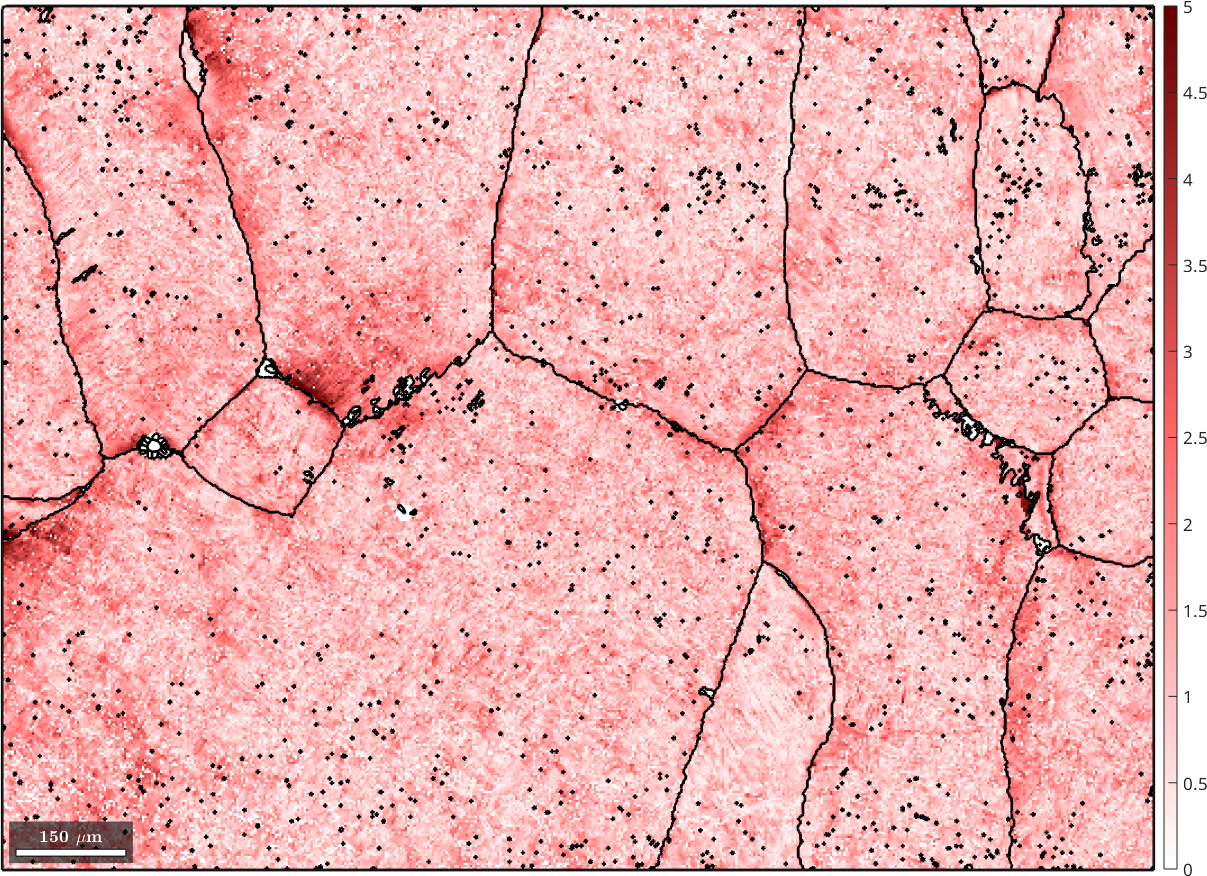

Lets finaly plot the reconstructed beta phase

plot(parentEBSD(betaName),ipfKey.orientation2color(parentEBSD(betaName).orientations),'figSize','large')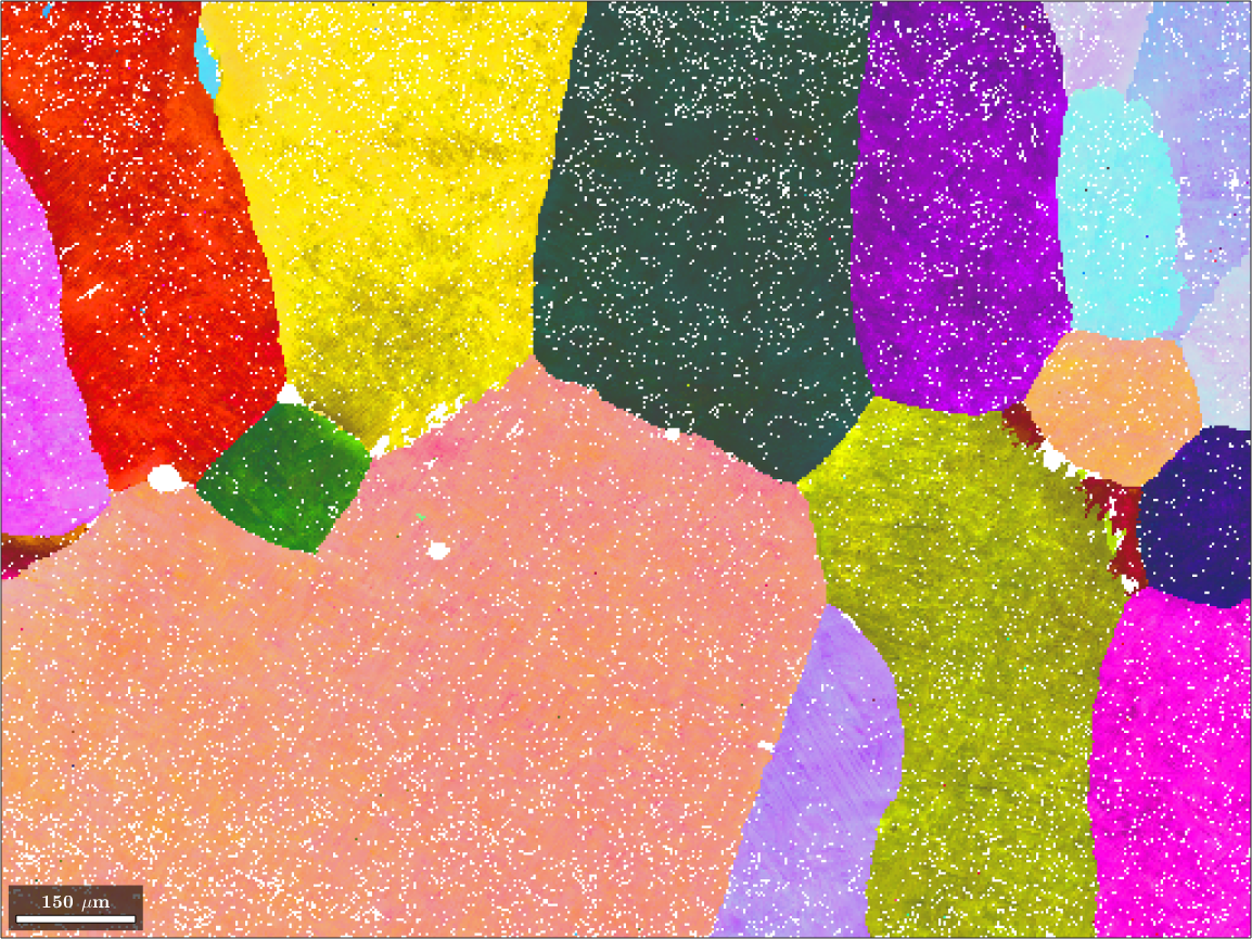

Denoising of the reconstructed beta phase

As promised we end our discussion by applying denoising techniques to fill the remaining holes of alpha grains. To this end we first reconstruct grains from the parent orientations and throw away all small grains

[parentGrains,parentEBSD.grainId] = calcGrains(parentEBSD('indexed'),'angle',5*degree);

% remove all the small grains
parentEBSD = parentEBSD(parentGrains(parentGrains.grainSize > 15));

% redo grain reconstruction
[parentGrains,parentEBSD.grainId] = calcGrains(parentEBSD('indexed'),'angle',5*degree);

% smooth the grains a bit
parentGrains = smooth(parentGrains,5);

Finally, we denoise the remaining beta orientations and at the same time fill the empty holes. We choose a very small smoothing parameter alpha to keep as many details as possible.

F= halfQuadraticFilter;
F.alpha = 0.1;
parentEBSD = smooth(parentEBSD,F,'fill',parentGrains);

% plot the resulting beta phase
plot(parentEBSD(betaName),ipfKey.orientation2color(parentEBSD(betaName).orientations),'figSize','large')

hold on
plot(parentGrains.boundary,'lineWidth',3)
hold off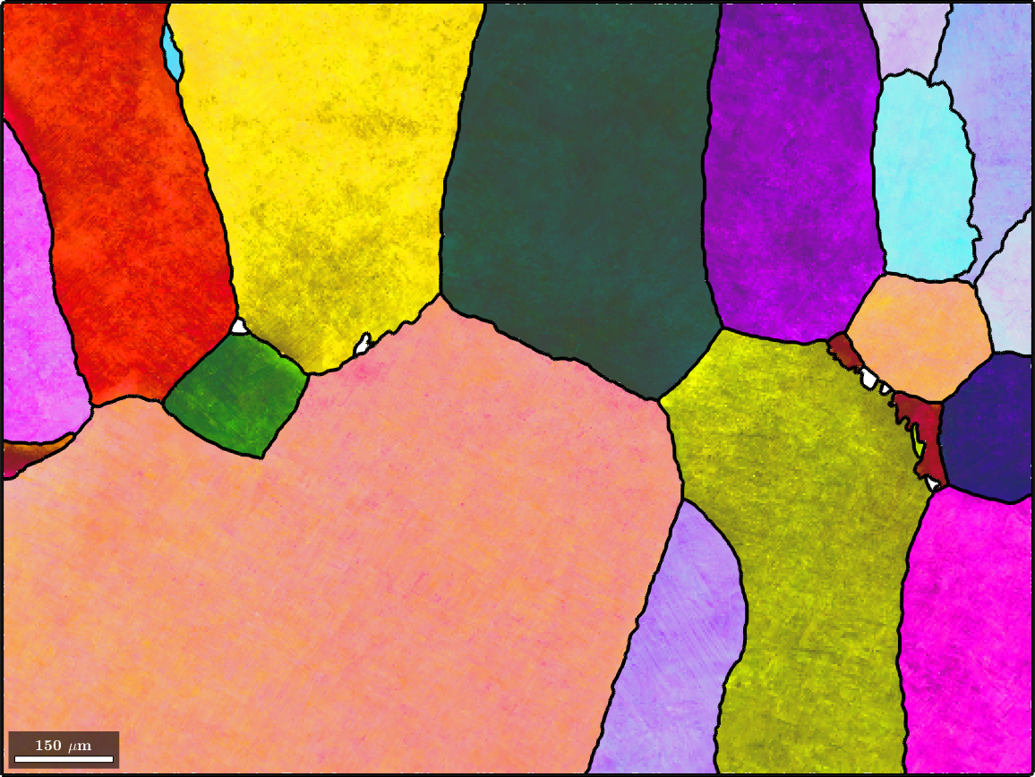

For comparison the map with original alpha phase and on top the recovered beta grain boundaries

plot(ebsd(alphaName),ebsd(alphaName).orientations,'figSize','large')

hold on
plot(parentGrains.boundary,'lineWidth',3)
hold off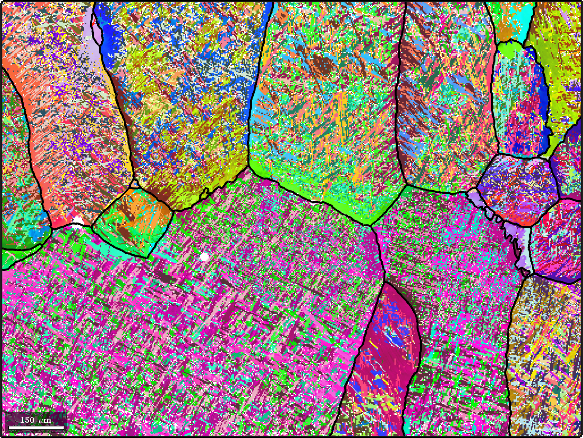

Summary of relevant thresholds

In parent grain reconstruction several parameters are involve are decicive for the success of the reconstruction

threshold for initial grain segmentation (1.5*degree)
maximum misfit at triple junctions (2.5 degree)
minimal misfit of the second best solution at triple junctions (2.5 degree)
minimum number of consistent votes (2)
threshold for merging beta grains (can be skipped)
threshold for merging alpha and beta grains (2.5 degree)

Visualize the misorientation to the mean reveals quite some fine structure in the reconstructed parent orientations.

cKey = axisAngleColorKey;
color = cKey.orientation2color(parentEBSD(betaName).orientations, parentGrains(parentEBSD(betaName).grainId).meanOrientation);
plot(parentEBSD(betaName),color)

hold on
plot(parentGrains.boundary,'lineWidth',3)
hold off